Load packages
# numerical calculation & data frames
import numpy as np
import pandas as pd

# visualization
import matplotlib.pyplot as plt
import seaborn as sns
import seaborn.objects as so

# pandas options
pd.set_option('mode.copy_on_write', True)  # pandas 2.0
pd.options.display.float_format = '{:.3f}'.format  # pd.reset_option('display.float_format')
# pd.options.display.max_rows = 7  # max number of rows to display

# NumPy options
np.set_printoptions(precision = 2, suppress=True)  # suppress scientific notation

# matplotlib options
from matplotlib import style
theme_dict = {**style.library['ggplot'], "grid.linestyle": ":", 'axes.facecolor': 'white', 'grid.color': '.6',}
so.Plot.config.theme.update(theme_dict)

# theme_dict = {**sns.axes_style("whitegrid"), "grid.linestyle": ":"}
# so.Plot.config.theme.update(theme_dict)

# For high resolution display
import matplotlib_inline
matplotlib_inline.backend_inline.set_matplotlib_formats("retina")
Cleaned Data
File: netflix_ratings.parquet
netflix = pd.read_parquet("data/netflix_ratings.parquet")
<class 'pandas.DataFrame'>
RangeIndex: 1862726 entries, 0 to 1862725
Data columns (total 7 columns):
 #   Column    Dtype
---  ------    -----
 0   movie_id  Int16
 1   user_id   Int32
 2   rating    Int8
 3   date      datetime64[ns]
 4   title     str
 5   genre     object
 6   year      int64
dtypes: Int16(1), Int32(1), Int8(1), datetime64[ns](1), int64(1), object(1), str(1)
memory usage: 100.7+ MB
| 0 |
3282 |
972104 |
4 |
2005-09-16 |
Sideways |
[Comedy, Drama, Romance] |
2004 |
| 1 |
143 |
2297762 |
5 |
2004-08-07 |
The Game |
[Drama, Mystery, Thriller] |
1997 |
| 2 |
1744 |
1489846 |
3 |
2003-05-22 |
Beverly Hills Cop |
[Action, Comedy, Crime] |
1984 |
| 3 |
357 |
1169994 |
5 |
2004-04-22 |
House of Sand and Fog |
[Crime, Drama] |
2003 |
| 4 |
3256 |
722964 |
3 |
2004-03-08 |
Swimming Pool |
[Crime, Drama, Mystery] |
2003 |
| ... |
... |
... |
... |
... |
... |
... |
... |
| 1862721 |
1585 |
813354 |
3 |
2005-02-09 |
Joy Ride |
[Action, Mystery, Thriller] |
2001 |
| 1862722 |
3782 |
1550938 |
3 |
2005-02-07 |
Flatliners |
[Drama, Horror, Sci-Fi] |
1990 |
| 1862723 |
3782 |
1550938 |
3 |
2005-02-07 |
Flatliners |
[Drama, Horror, Mystery] |
1990 |
| 1862724 |
483 |
868452 |
3 |
2003-09-29 |
Rush Hour 2 |
[Action, Comedy, Crime] |
2001 |
| 1862725 |
2782 |
1465983 |
4 |
2005-06-22 |
Braveheart |
[Biography, Drama, War] |
1995 |
1862726 rows × 7 columns
Data Wrangling
대략 다음과 같은 transform들을 조합하여 분석에 필요한 상태로 바꿈
- 변수들(열)과 관측치(행)를 선택:
subsetting
- 조건에 맞는 부분(관측치, 행)만 필터링:
query()
- 조건에 맞도록 행을 재정렬:
sort_values()
- 변수들과 함수들을 이용하여 새로운 변수를 생성:
assign()
- 카테고리별로 나뉘어진 데이터에 대한 통계치를 생성:
groupby(), agg(), apply()
netflix_1990 = (
    netflix
    .loc[:, ["title", "rating", "date", "year"]]
    .query("year >= 1990")
    .assign(
        decade=lambda x: x["year"] // 10 * 10,  # 10년 단위
        weekday=lambda x: x["date"].dt.day_name().str[:3]  # 요일
    )
    .sort_values("year")
)
netflix_1990
| 150148 |
Flatliners |
3 |
2004-08-14 |
1990 |
1990 |
Sat |
| 1269856 |
Look Who's Talking Too |
3 |
2004-09-24 |
1990 |
1990 |
Fri |
| 562709 |
Ghost |
2 |
2004-12-28 |
1990 |
1990 |
Tue |
| 1667117 |
The Grifters |
3 |
2005-05-15 |
1990 |
1990 |
Sun |
| 1269834 |
Ghost |
4 |
2002-03-01 |
1990 |
1990 |
Fri |
| ... |
... |
... |
... |
... |
... |
... |
| 456802 |
Beauty Shop |
5 |
2005-10-22 |
2005 |
2000 |
Sat |
| 608408 |
Hostage |
4 |
2005-10-10 |
2005 |
2000 |
Mon |
| 456776 |
Hostage |
5 |
2005-07-18 |
2005 |
2000 |
Mon |
| 1818277 |
Coach Carter |
4 |
2005-08-03 |
2005 |
2000 |
Wed |
| 519199 |
The Hitchhiker's Guide to the Galaxy |
3 |
2005-11-22 |
2005 |
2000 |
Tue |
1496107 rows × 6 columns
subsetting
변수들(열)과 관측치(행)를 선택
query()
조건에 맞는 부분(관측치, 행)만 필터링
sort_values()
조건에 맞도록 행을 재정렬
assign()
변수들과 함수들을 이용하여 새로운 변수를 생성
groupby(), agg(), apply()
카테고리별로 나뉘어진 데이터에 대한 통계치를 생성
Exploratory Data Analysis (EDA)
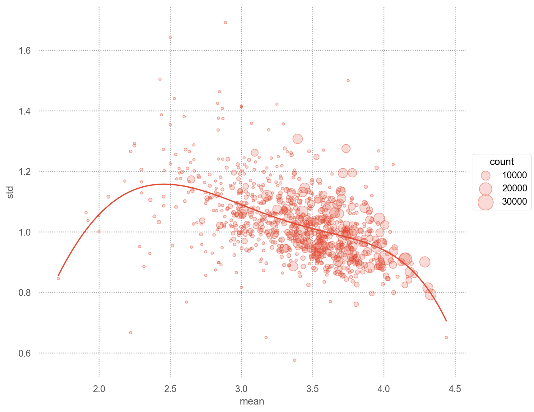
평점 분포
mean_ratings = (
    netflix
    .groupby(["title"])["rating"]
    .agg(["mean", "std", "count"])
    .reset_index()
)
mean_ratings
| 0 |
10 |
3.104 |
0.956 |
498 |
| 1 |
10 Things I Hate About You |
3.728 |
0.992 |
4705 |
| 2 |
11:14 |
3.203 |
1.030 |
266 |
| 3 |
13 Ghosts |
3.557 |
1.129 |
758 |
| 4 |
1984 |
3.367 |
1.131 |
488 |
| ... |
... |
... |
... |
... |
| 820 |
Wonder Boys |
3.552 |
0.968 |
3278 |
| 821 |
Wonderland |
3.000 |
1.098 |
152 |
| 822 |
Wrongfully Accused |
3.290 |
1.143 |
252 |
| 823 |
Yellow Submarine |
3.575 |
1.105 |
784 |
| 824 |
Youngblood |
3.256 |
1.029 |
328 |
825 rows × 4 columns
mean_ratings.sort_values("mean", ascending=False)
| 430 |
Paradise Lost: The Child Murders at Robin Hood... |
4.440 |
0.651 |
25 |
| 734 |
The Sixth Sense |
4.329 |
0.793 |
15166 |
| 733 |
The Silence of the Lambs |
4.310 |
0.815 |
12940 |
| 101 |
Braveheart |
4.289 |
0.901 |
13590 |
| 72 |
Batman Begins |
4.215 |
0.860 |
5529 |
| ... |
... |
... |
... |
... |
| 641 |
The Gunman |
2.000 |
1.000 |
13 |
| 306 |
Inseminoid |
2.000 |
1.054 |
10 |
| 468 |
Red Riding Hood |
1.923 |
1.038 |
13 |
| 476 |
Rhinestone |
1.909 |
1.063 |
66 |
| 562 |
Stuck on You |
1.714 |
0.845 |
21 |
825 rows × 4 columns
(
    so.Plot(mean_ratings, x="mean", y="std")
    .add(so.Dots(alpha=.5), pointsize="count")
    .add(so.Line(), so.PolyFit(5))
    .scale(pointsize=(3, 20))
    .layout(size=(8, 7))
)
netflix2 = (
    netflix
    .assign(
        decade=lambda x: x["year"] // 10 * 10,  # 10년 단위
        weekday=lambda x: x["date"].dt.day_name().str[:3],
        weekend=lambda x: x["weekday"].isin(["Sat", "Sun"]),
        title_length=lambda x: x["title"].str.len()
    )
)

netflix2["weekday"] = netflix2["weekday"].astype("category").cat.set_categories(["Mon", "Tue", "Wed", "Thu", "Fri", "Sat", "Sun"])

mean_ratings_by_wday = (
    netflix2
    .groupby(["weekday"], observed=True)["rating"]
    .agg(["mean", "std", "count"])
    .reset_index()
)
mean_ratings_by_wday
| 0 |
Mon |
3.584 |
1.054 |
324006 |
| 1 |
Tue |
3.582 |
1.054 |
331272 |
| 2 |
Wed |
3.590 |
1.055 |
311012 |
| 3 |
Thu |
3.593 |
1.057 |
267394 |
| 4 |
Fri |
3.589 |
1.061 |
245186 |
| 5 |
Sat |
3.596 |
1.065 |
184385 |
| 6 |
Sun |
3.596 |
1.060 |
199471 |
요일별 평점
(
    so.Plot(mean_ratings_by_wday, x="weekday", y="mean")
    .add(so.Dot(), pointsize="count")
)
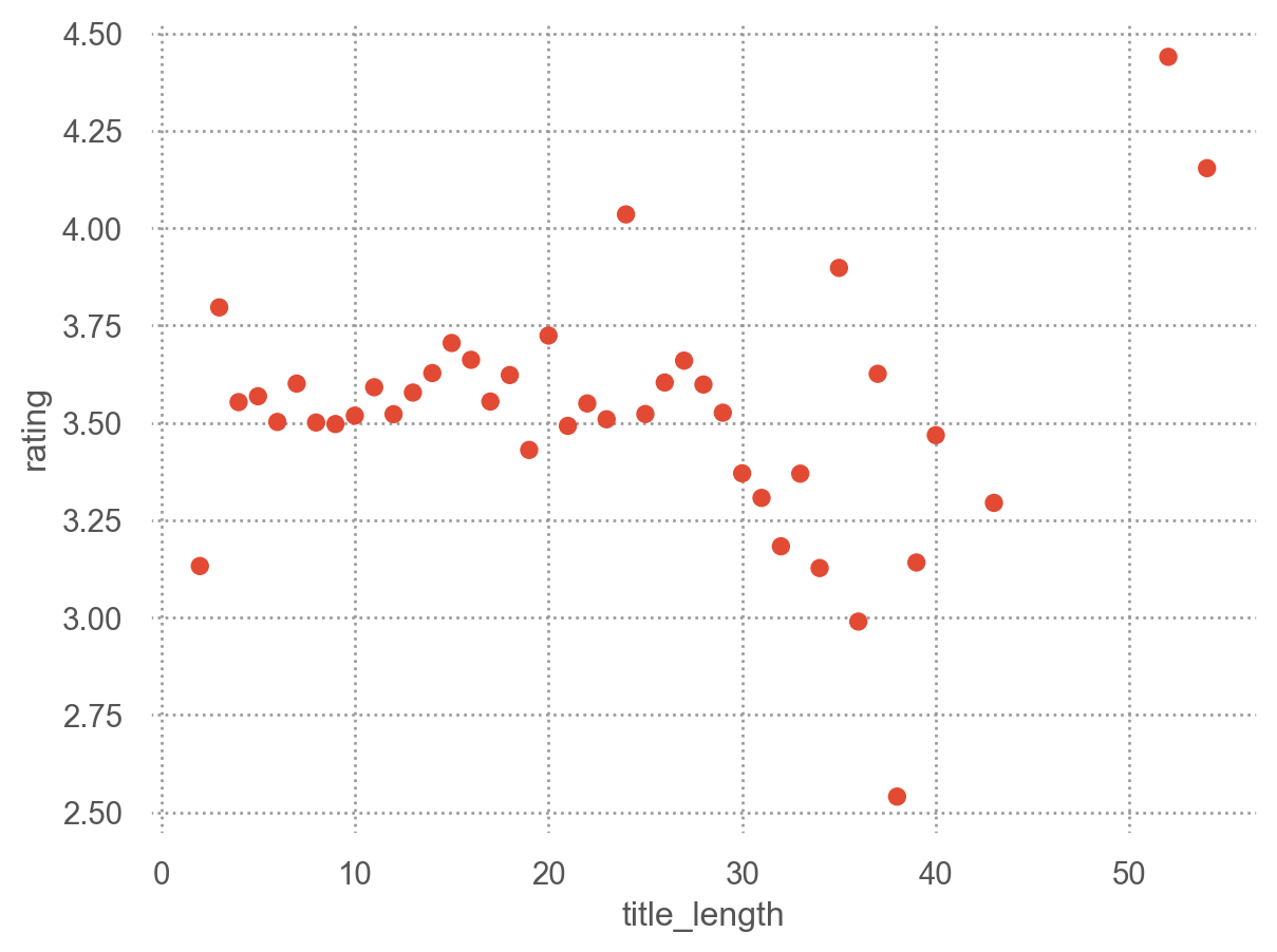
제목의 길이?
(
    so.Plot(netflix2, x="title_length", y="rating")
    .add(so.Dot(), so.Agg("mean"))
)
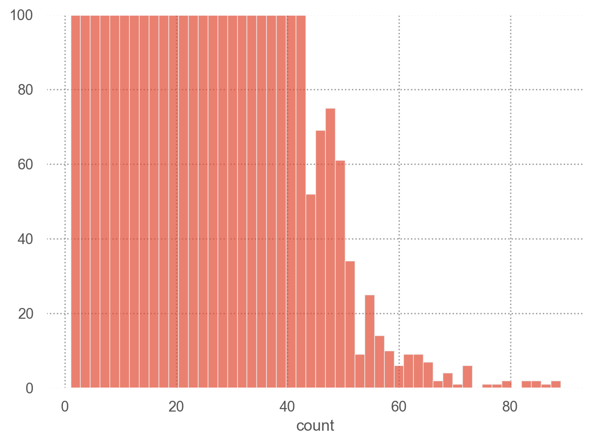
시청자별 분석
viewing_count = netflix.groupby("user_id")["rating"].size()
viewing_count
user_id
6          15
7          15
10          4
33          2
59          6
           ..
2649384     1
2649388     8
2649401     5
2649426     3
2649429     6
Name: rating, Length: 336915, dtype: Int64
# pandas의 method를 사용한 시각화
viewing_count.hist(bins=100);
viewing_count_df = viewing_count.reset_index(name="count")
(
    so.Plot(viewing_count_df, x="count")
    .add(so.Bars(), so.Hist(bins=50))
    .limit(y=(0, 100))
)
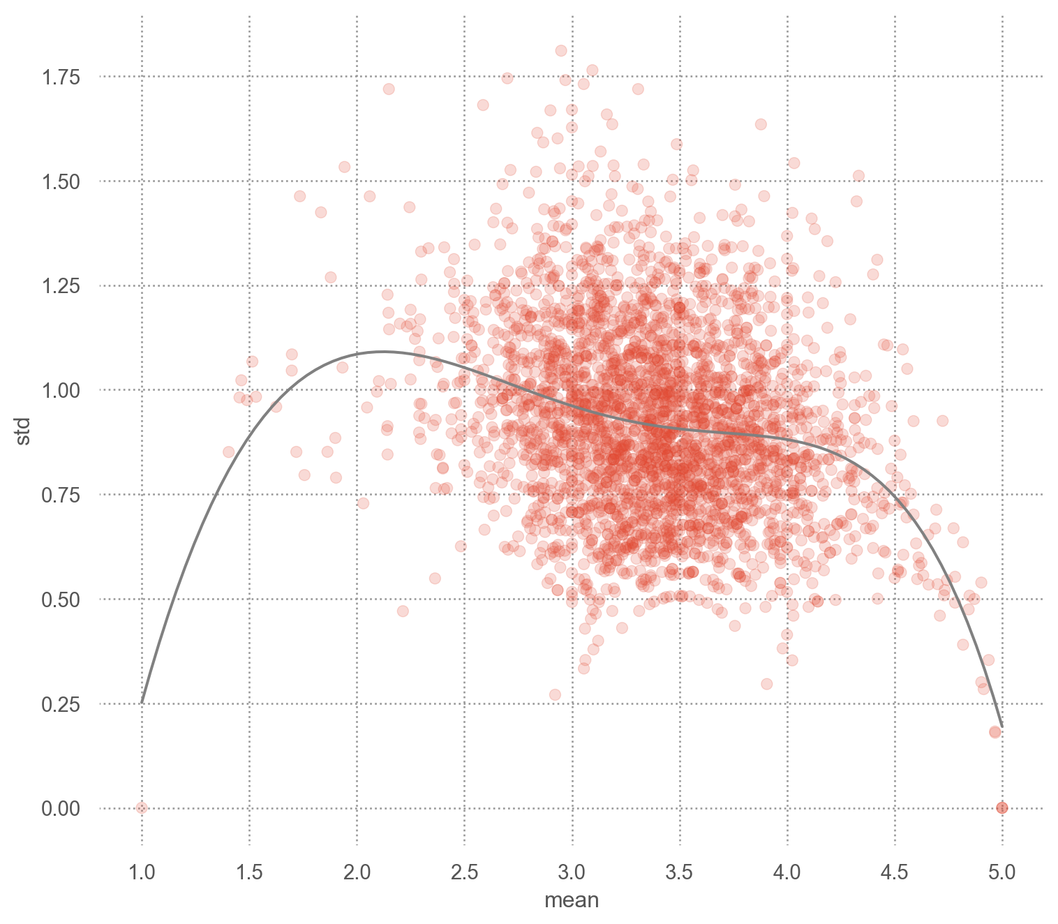
user_stats = (
    netflix
    .groupby("user_id")["rating"]
    .agg(["mean", "std", "count"])
)
user_stats
| user_id |
|
|
|
| 6 |
3.200 |
0.414 |
15 |
| 7 |
4.067 |
1.033 |
15 |
| 10 |
3.500 |
1.732 |
4 |
| 33 |
3.500 |
0.707 |
2 |
| 59 |
4.000 |
1.549 |
6 |
| ... |
... |
... |
... |
| 2649384 |
3.000 |
<NA> |
1 |
| 2649388 |
3.125 |
0.835 |
8 |
| 2649401 |
4.200 |
1.095 |
5 |
| 2649426 |
3.667 |
0.577 |
3 |
| 2649429 |
4.000 |
0.894 |
6 |
336915 rows × 3 columns
user_stat_30 = user_stats.query("count >= 30")
user_stat_30
| user_id |
|
|
|
| 1333 |
2.674 |
0.778 |
43 |
| 2213 |
3.871 |
0.846 |
31 |
| 2455 |
3.433 |
0.817 |
30 |
| 2905 |
3.700 |
1.418 |
30 |
| 3321 |
2.977 |
1.012 |
43 |
| ... |
... |
... |
... |
| 2645579 |
3.935 |
0.680 |
46 |
| 2646347 |
3.263 |
1.032 |
38 |
| 2646574 |
3.119 |
0.803 |
42 |
| 2647197 |
3.389 |
1.153 |
36 |
| 2648287 |
3.600 |
0.847 |
35 |
3051 rows × 3 columns
(
    so.Plot(user_stat_30, x="mean", y="std")
    .add(so.Dot(alpha=.2))
    .add(so.Line(color=".5"), so.PolyFit(5))
    .layout(size=(8, 7))
)
장르별 분석
0             [Comedy, Drama, Romance]
1           [Drama, Mystery, Thriller]
2              [Action, Comedy, Crime]
3                       [Crime, Drama]
4              [Crime, Drama, Mystery]
                      ...
1862721    [Action, Mystery, Thriller]
1862722        [Drama, Horror, Sci-Fi]
1862723       [Drama, Horror, Mystery]
1862724        [Action, Comedy, Crime]
1862725        [Biography, Drama, War]
Name: genre, Length: 1862726, dtype: object
netflix_long = netflix.explode('genre')
| 0 |
3282 |
972104 |
4 |
2005-09-16 |
Sideways |
Comedy |
2004 |
| 0 |
3282 |
972104 |
4 |
2005-09-16 |
Sideways |
Drama |
2004 |
| 0 |
3282 |
972104 |
4 |
2005-09-16 |
Sideways |
Romance |
2004 |
| 1 |
143 |
2297762 |
5 |
2004-08-07 |
The Game |
Drama |
1997 |
| 1 |
143 |
2297762 |
5 |
2004-08-07 |
The Game |
Mystery |
1997 |
| ... |
... |
... |
... |
... |
... |
... |
... |
| 1862724 |
483 |
868452 |
3 |
2003-09-29 |
Rush Hour 2 |
Comedy |
2001 |
| 1862724 |
483 |
868452 |
3 |
2003-09-29 |
Rush Hour 2 |
Crime |
2001 |
| 1862725 |
2782 |
1465983 |
4 |
2005-06-22 |
Braveheart |
Biography |
1995 |
| 1862725 |
2782 |
1465983 |
4 |
2005-06-22 |
Braveheart |
Drama |
1995 |
| 1862725 |
2782 |
1465983 |
4 |
2005-06-22 |
Braveheart |
War |
1995 |
4806517 rows × 7 columns
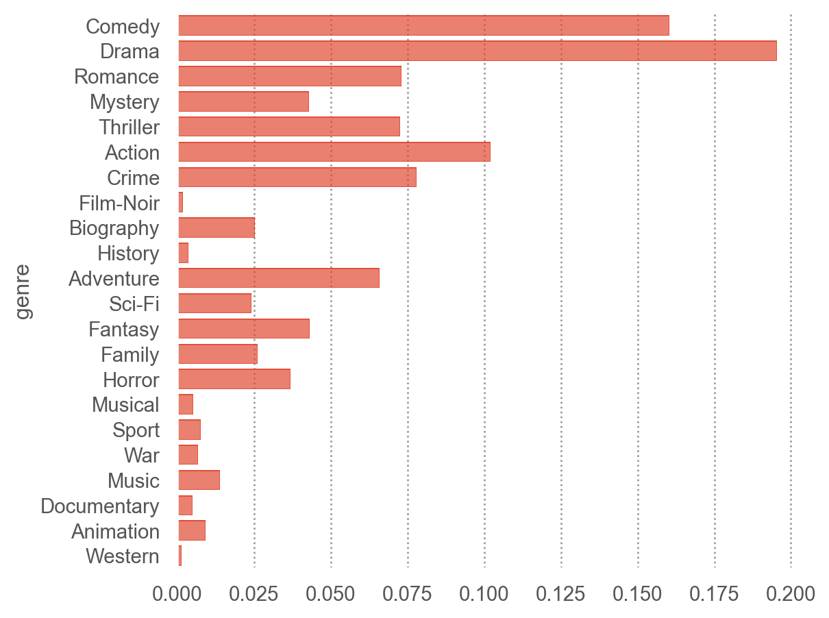
(
    so.Plot(netflix_long, y="genre")  # y에 genre가 나오도록!
    .add(so.Bar(), so.Hist("proportion"))
)
genre_mean = (
    netflix_long
    .groupby('genre')['rating']
    .agg(['mean', 'std', 'count'])
    .reset_index()
)
genre_mean
| 0 |
Action |
3.557 |
1.050 |
490601 |
| 1 |
Adventure |
3.576 |
1.064 |
316881 |
| 2 |
Animation |
3.811 |
1.018 |
44297 |
| 3 |
Biography |
3.878 |
0.995 |
121688 |
| 4 |
Comedy |
3.528 |
1.067 |
770697 |
| 5 |
Crime |
3.624 |
1.043 |
374283 |
| 6 |
Documentary |
3.810 |
1.070 |
23833 |
| 7 |
Drama |
3.661 |
1.045 |
939328 |
| 8 |
Family |
3.588 |
1.057 |
125263 |
| 9 |
Fantasy |
3.552 |
1.057 |
207485 |
| 10 |
Film-Noir |
3.965 |
0.935 |
9020 |
| 11 |
History |
3.550 |
1.014 |
16961 |
| 12 |
Horror |
3.386 |
1.065 |
177556 |
| 13 |
Music |
3.683 |
1.084 |
66609 |
| 14 |
Musical |
3.616 |
1.033 |
24462 |
| 15 |
Mystery |
3.577 |
1.043 |
206452 |
| 16 |
Romance |
3.566 |
1.053 |
351176 |
| 17 |
Sci-Fi |
3.332 |
1.090 |
115480 |
| 18 |
Sport |
3.687 |
0.994 |
36883 |
| 19 |
Thriller |
3.620 |
1.030 |
348897 |
| 20 |
War |
3.908 |
1.037 |
32304 |
| 21 |
Western |
3.577 |
1.045 |
6361 |
genre_mean.nlargest(3, "mean")
| 10 |
Film-Noir |
3.965 |
0.935 |
9020 |
| 20 |
War |
3.908 |
1.037 |
32304 |
| 3 |
Biography |
3.878 |
0.995 |
121688 |
order_by_mean = genre_mean.sort_values("mean", ascending=False)["genre"].values

(
    so.Plot(genre_mean, y="genre", x="mean")
    .add(so.Bar())
    .scale(y=so.Nominal(order=order_by_mean))  # 그래프에 순서 부여
    .limit(x=(3, 4.1))
)
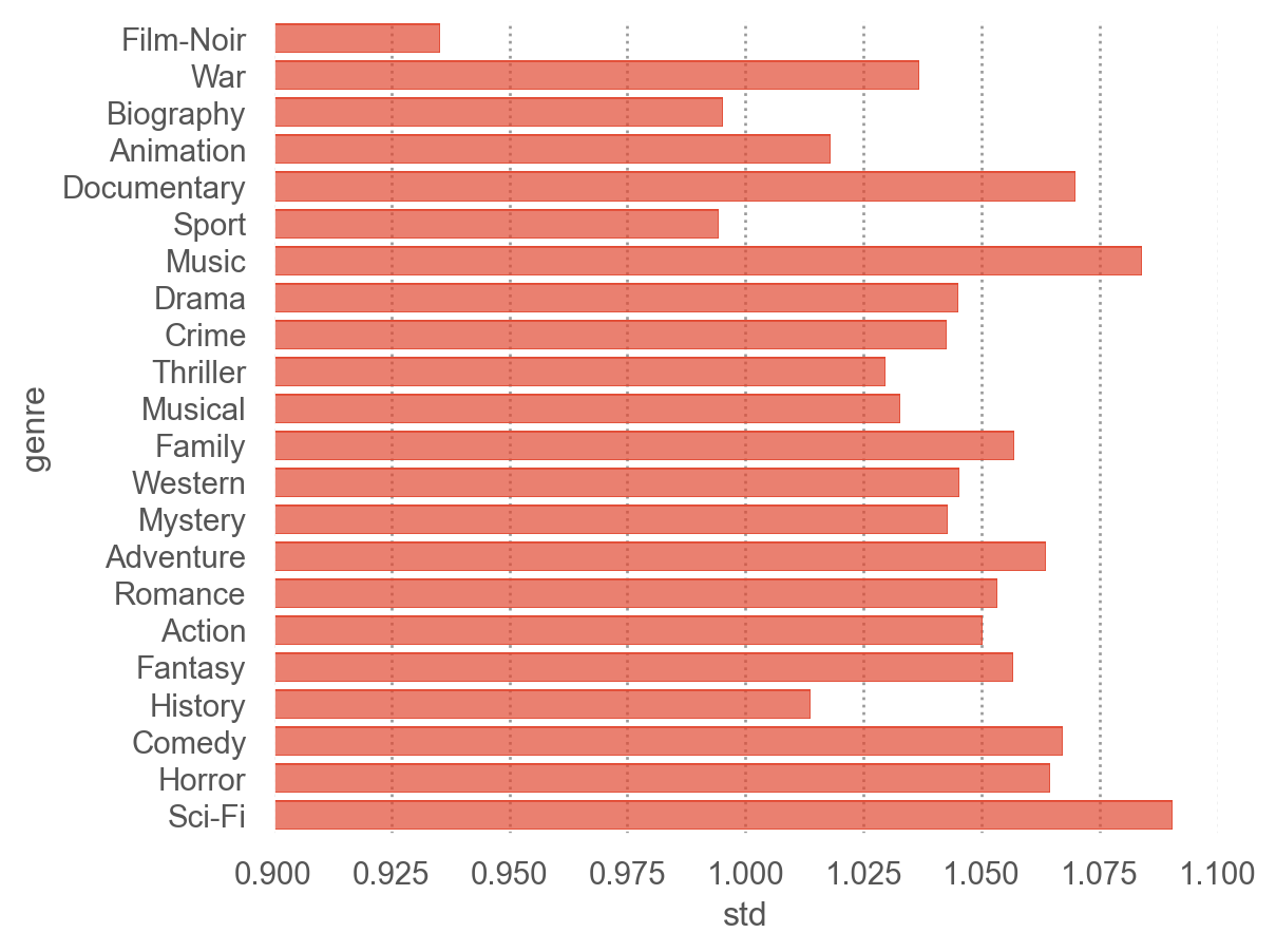
(
    so.Plot(genre_mean, y="genre", x="std")
    .add(so.Bar())
    .scale(y=so.Nominal(order=order_by_mean))  # 그래프에 순서 부여
    .limit(x=(.9, 1.1))
)
netflix_long["weekday"] = netflix_long["date"].dt.day_name().str[:3]
netflix_long["weekday"] = netflix_long["weekday"].astype("category").cat.set_categories(["Mon", "Tue", "Wed", "Thu", "Fri", "Sat", "Sun"])

genre_mean_by_weekday = (
    netflix_long
    .groupby(['genre', 'weekday'], observed=True)['rating']
    .agg(['mean', 'std', 'count'])
    .reset_index()
)
genre_mean_by_weekday
| 0 |
Action |
Mon |
3.555 |
1.045 |
85715 |
| 1 |
Action |
Tue |
3.549 |
1.043 |
86670 |
| 2 |
Action |
Wed |
3.561 |
1.047 |
82093 |
| 3 |
Action |
Thu |
3.556 |
1.051 |
70626 |
| 4 |
Action |
Fri |
3.548 |
1.059 |
64562 |
| ... |
... |
... |
... |
... |
... |
| 149 |
Western |
Wed |
3.579 |
1.043 |
1017 |
| 150 |
Western |
Thu |
3.621 |
1.063 |
931 |
| 151 |
Western |
Fri |
3.581 |
1.034 |
836 |
| 152 |
Western |
Sat |
3.555 |
1.015 |
632 |
| 153 |
Western |
Sun |
3.602 |
0.997 |
738 |
154 rows × 5 columns
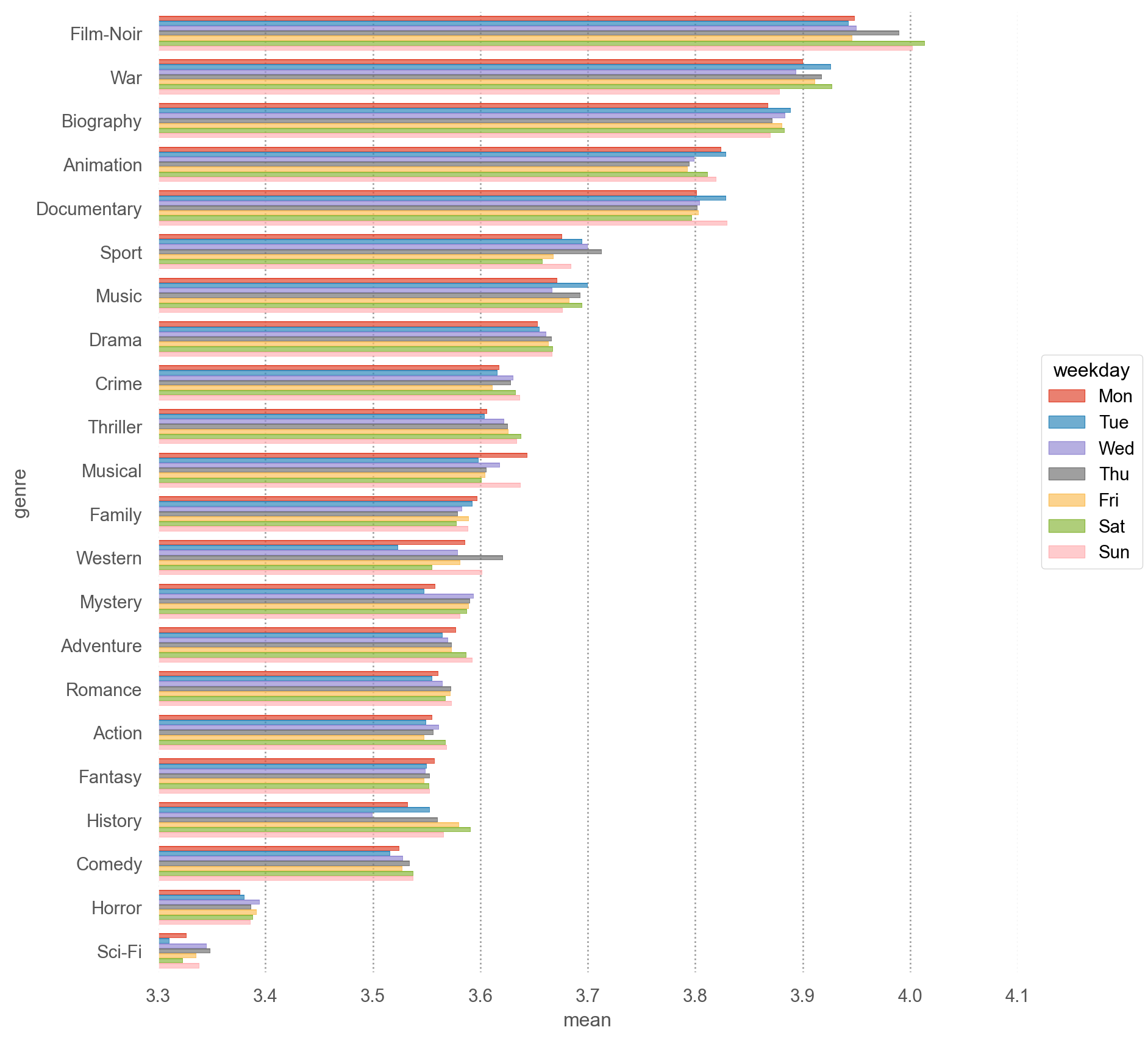
order_by_mean = genre_mean.sort_values("mean", ascending=False)["genre"].values

(
    so.Plot(genre_mean_by_weekday, y="genre", x="mean", color="weekday")
    .add(so.Bar(), so.Dodge())
    .scale(y=so.Nominal(order=order_by_mean))  # 그래프에 순서 부여
    # .facet("weekday")
    .limit(x=(3.3, 4.1))
    .layout(size=(9, 9))
)
mean_ratings_by_genre = (
    netflix_long
    .groupby(["title", "genre"])["rating"]
    .agg(["mean", "std", "count"])
    .reset_index()
)
mean_ratings_by_genre
| 0 |
10 |
Comedy |
3.104 |
0.956 |
498 |
| 1 |
10 |
Romance |
3.104 |
0.956 |
498 |
| 2 |
10 Things I Hate About You |
Comedy |
3.728 |
0.992 |
4705 |
| 3 |
10 Things I Hate About You |
Drama |
3.728 |
0.992 |
4705 |
| 4 |
10 Things I Hate About You |
Romance |
3.728 |
0.992 |
4705 |
| ... |
... |
... |
... |
... |
... |
| 2199 |
Yellow Submarine |
Animation |
3.575 |
1.105 |
784 |
| 2200 |
Yellow Submarine |
Comedy |
3.575 |
1.105 |
784 |
| 2201 |
Youngblood |
Drama |
3.256 |
1.029 |
328 |
| 2202 |
Youngblood |
Romance |
3.256 |
1.029 |
328 |
| 2203 |
Youngblood |
Sport |
3.256 |
1.029 |
328 |
2204 rows × 5 columns
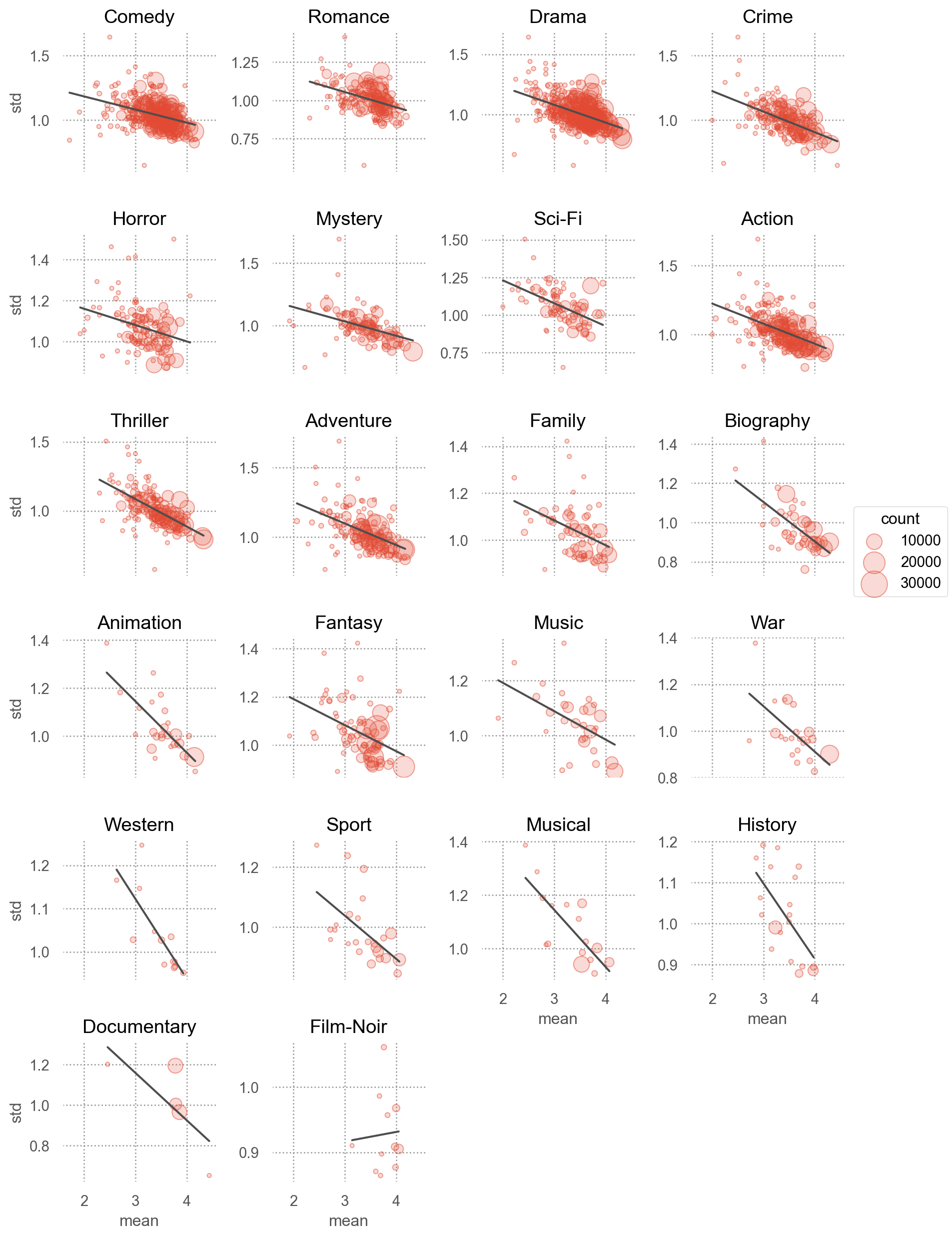
(
    so.Plot(mean_ratings_by_genre, x="mean", y="std")
    .add(so.Dots(alpha=.5), pointsize="count")
    .add(so.Line(color=".3"), so.PolyFit(1))
    .facet("genre", wrap=4)
    .share(y=False)
    .scale(pointsize=(3, 20))
    .layout(size=(9, 13))
)
출시년도
| 0 |
3282 |
972104 |
4 |
2005-09-16 |
Sideways |
[Comedy, Drama, Romance] |
2004 |
| 1 |
143 |
2297762 |
5 |
2004-08-07 |
The Game |
[Drama, Mystery, Thriller] |
1997 |
| 2 |
1744 |
1489846 |
3 |
2003-05-22 |
Beverly Hills Cop |
[Action, Comedy, Crime] |
1984 |
netflix.groupby(["year", "title"])["rating"].agg(["mean", "count"])
| year |
title |
|
|
| 1916 |
20,000 Leagues Under the Sea |
3.704 |
162 |
| 1918 |
Chaplin |
3.000 |
47 |
| 1922 |
Robin Hood |
3.080 |
75 |
| 1927 |
It |
4.067 |
15 |
| The Little Rascals |
3.789 |
114 |
| ... |
... |
... |
... |
| 2005 |
The Amityville Horror |
3.502 |
1947 |
| The Ballad of Jack and Rose |
2.971 |
313 |
| The Hitchhiker's Guide to the Galaxy |
2.997 |
2949 |
| The Pacifier |
3.580 |
3966 |
| Unleashed |
3.733 |
845 |
844 rows × 2 columns
(
    so.Plot(netflix, x="year", y="rating")
    .add(so.Line(marker="."), so.Agg("mean"))
)
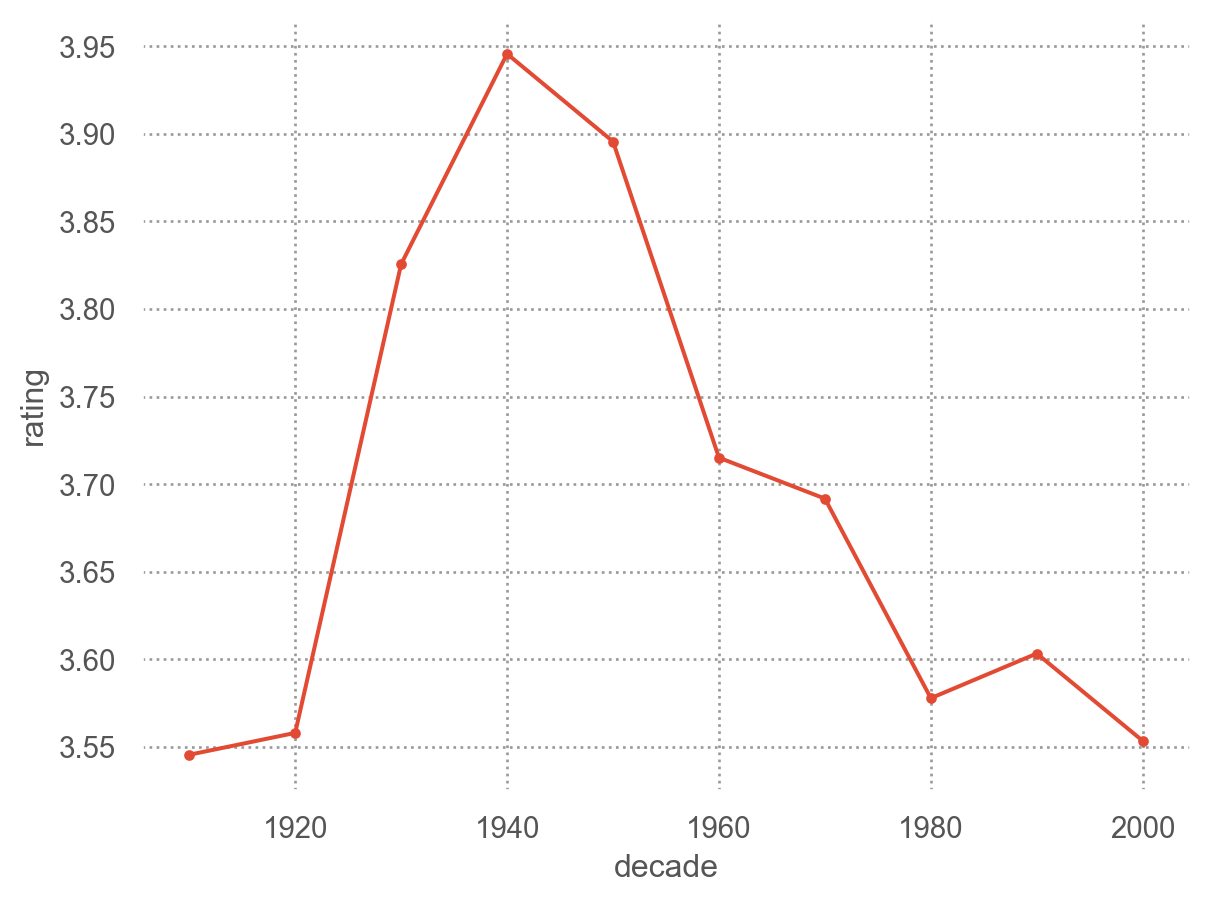
# 10년 단위로
netflix["decade"] = netflix["year"] // 10 * 10
(
    so.Plot(netflix, x="decade", y="rating")
    .add(so.Line(marker="."), so.Agg("mean"))
)