Python Programming
  • Home
  • Intro
    • History & Background
    • Python Setup
  • QPB
    • Part I: Chapter 1-3
    • Part II
    • 5. Lists, Tuples, Sets
  • Exercises
    • Chapter 5: Lists, Tuples, Sets
    • Chapter 6: Strings
    • Chapter 7: Dictionaries
    • Chapter 8: Control flow
    • Chapter 9: Functions
    • Chapter 14: Exceptions
    • Chapter 15: Classes
  • Exploring Data
    • NumPy & pandas
    • Visualization
  • Library System
  • Netflix Movie Analysis
    • Notes
    • Project-Native
    • Project-pandas
  • References
    • QPB Part 1
    • QPB Part 2
    • QPB Part 3
    • QPB Part 4

On this page

  • NumPy
    • Python vs. NumPy 연산
  • pandas
    • Series
    • DataFrame
  • Vectorized operation

NumPy and pandas

Load packages
import numpy as np
import pandas as pd

# pandas options
pd.set_option('mode.copy_on_write', True)  # pandas 2.0
pd.options.display.float_format = '{:.2f}'.format  # pd.reset_option('display.float_format')
pd.options.display.max_rows = 7  # max number of rows to display

# NumPy options
np.set_printoptions(precision = 2, suppress=True)  # suppress scientific notation

Numpy & pandas

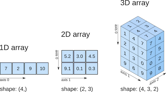
Python 언어는 수치 계산을 위해 디자인되지 않았기 때문에, 데이터 분석에 대한 효율적이고 빠른 계산이 요구되면서 C/C++이라는 언어로 구현된 NumPy (Numerical Python)가 탄생하였고, Python 생태계 안에 통합되었음. 기본적으로 Python 언어 안에 새로운 언어라고 볼 수 있음. 데이터 사이언스에서의 대부분의 계산은 NumPy의 ndarray (n-dimensioal array)와 수학적 operator들을 통해 계산됨.

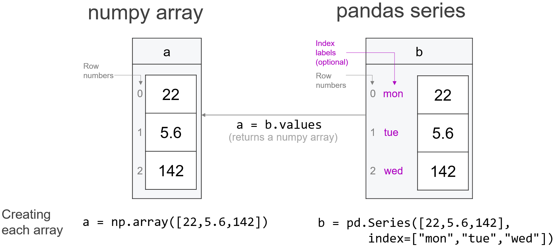
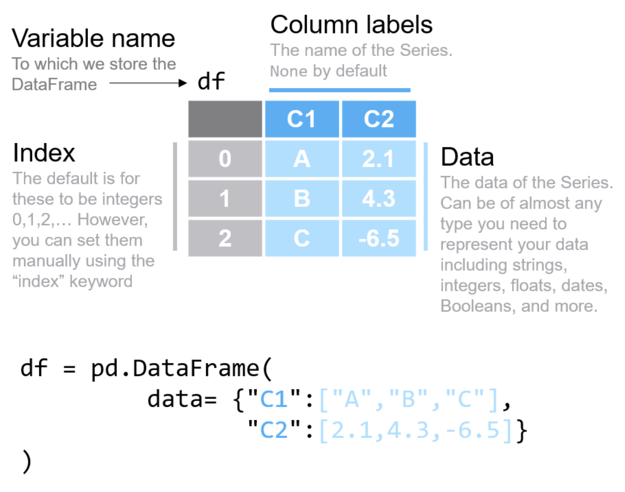
데이터 사이언스가 발전함에 따라 단일한 floating-point number들을 성분으로하는 array들의 계산에서 벗어나 칼럼별로 다른 데이터 타입(string, integer, object..)을 포함하는 tabular 형태의 데이터를 효율적으로 처리해야 할 필요성이 나타났고, 이를 다룰 수 있는 새로운 언어를 NumPy 위에 개발한 것이 pandas임. 이는 기본적으로 Wes Mckinney에 의해 독자적으로 개발이 시작되었으며, 디자인적으로 불만족스러운 점이 지적되고는 있으나 데이터 사이언스의 기본적인 언어가 되었음.

NumPy와 pandas에 대한 자세한 내용은 Python for Data Analysis, 3E by Wes McKinney 참고

NumPy는 Ch.4 & appendices

NumPy

  • 수학적 symbolic 연산에 대한 구현이라고 볼 수 있으며,
  • 행렬(matrix) 또는 벡터(vector)를 ndarray (n-dimensional array)이라는 이름으로 구현함.
    • 사실상 정수(int)나 실수(float)의 한가지 타입으로 이루어짐.
    • 고차원의 arrays 가능
  • 가령, 다음과 같은 행렬 연산이 있다면,
    \(\begin{bmatrix}1 & 2 \\ 3 & 4 \\ 5 & 6 \end{bmatrix} \begin{bmatrix}2 \\ -1 \end{bmatrix} = \begin{bmatrix}0 \\ 2 \\ 4 \end{bmatrix}\)


A = np.array([[1, 2],
              [3, 4],
              [5, 6]]) # 3x2 matrix
X = np.array([[2],
              [-1]]) # 2x1 matrix

A.dot(X)  # 또는 A @ X: matrix multiplication
array([[0],
       [2],
       [4]])

Vector vs. Matrix

arr_1d = np.array([0, 2, 4]) # 1-dim array: vector
arr_1d.reshape(3, 1) # 3x1 matrix
array([[0],
       [2],
       [4]])

자연스러운 연산 가능

A + A      # element-wise addition
2 * A - 1  # braodcasting
np.exp(A)  # element-wise

Python vs. NumPy 연산

a = 2**31 - 1
print(a)
print(a + 1)
2147483647
2147483648
a = np.array([2**31 - 1], dtype='int32')
print(a)
print(a + 1)
[2147483647]
[-2147483648]

계산의 효율성을 위해 여러 데이터 타입이 존재

Source: Ch.4 in Python for Data Analysis (3e) by Wes McKinney

pandas

Series & DataFrame

Series

1개의 칼럼으로 이루어진 데이터 포멧: 1d numpy array에 labels을 부여한 것으로 볼 수 있음.
DataFrame의 각 칼럼들을 Series로 이해할 수 있음.

Source: Practical Data Science

DataFrame

각 칼럼들이 한 가지 데이터 타입으로 이루어진 tabular형태 (2차원)의 데이터 포맷

  • 각 칼럼은 기본적으로 한 가지 데이터 타입인 것이 이상적이나, 다른 타입이 섞여 있을 수 있음
  • NumPy의 2차원 array의 각 칼럼에 labels을 부여한 것으로 볼 수도 있으나, 여러 다른 기능들이 추가됨
  • NumPy의 경우 고차원의 array를 다룰 수 있음: ndarray
    • 고차원의 DataFrame과 비슷한 것은 xarray가 존재
  • Labels와 index를 제외한 데이터 값은 거의 NumPy ndarray로 볼 수 있음
    (pandas.array 존재)

Source: Practical Data Science


ndarray <> DataFrame

df = pd.DataFrame(A, columns=["A1", "A2"])
df
   A1  A2
0   1   2
1   3   4
2   5   6
# 데이터 값들은 NumPy array
df.values # 또는 df.to_numpy()
array([[1, 2],
       [3, 4],
       [5, 6]])
type(df)
pandas.core.frame.DataFrame

DataFrame의 연산

NumPy의 ndarray들이 연산되는 방식과 동일하게 series나 DataFrame들의 연산 가능함

df + 2 * df
np.log(df)

NumPy의 데이터 타입을 확장

pandas extension types

Vectorized operation

반복문을 명시적으로 작성하지 않고도 배열 전체에 대해 연산이 수행 가능

Python의 기본 리스트를 사용할 때는 각 요소에 대해 반복문(for loop)이나 list comprehension을 사용해야 하지만, NumPy의 vectorized operation은

  1. 속도: 수십 배에서 수백 배까지 빠름
  2. 코드 간결성: 반복문 없이 수학적 표현 그대로 작성 가능
  3. 메모리 효율성: 내부적으로 최적화된 메모리 접근

vectorized operation이 빠른 이유

  1. Pre-compiled C code: NumPy의 내부 연산은 C/C++로 작성되어 컴파일된 코드로 실행됨
  2. Contiguous memory: 데이터가 메모리에 연속적으로 배치되어 있어 캐시 효율성이 높음
  3. SIMD (Single Instruction, Multiple Data): 현대 CPU의 벡터 연산 명령어를 활용하여 한 번의 명령으로 여러 데이터를 동시에 처리
  4. No Python overhead: Python interpreter의 오버헤드(타입 체크, 함수 호출 등)를 반복하지 않음

반면, Python의 list comprehension은: - 각 요소마다 Python interpreter를 거쳐야 함 - 타입 체크와 메모리 할당이 반복적으로 발생 - 최적화되지 않은 메모리 접근 패턴

제곱 계산 비교

# 큰 데이터 생성
n = 1_000_000
python_list = list(range(n))
numpy_array = np.arange(n)

print(f"python_list: {python_list[:10]}")
print(f"numpy_array: {numpy_array[:10]}")
python_list: [0, 1, 2, 3, 4, 5, 6, 7, 8, 9]
numpy_array: [0 1 2 3 4 5 6 7 8 9]
# Python list comprehension
time_list = %timeit -o [x**2 for x in python_list]

# NumPy vectorized operation
time_numpy = %timeit -o numpy_array**2

print(f"\n속도 향상: {time_list.average / time_numpy.average:.1f}배")
32.8 ms ± 747 μs per loop (mean ± std. dev. of 7 runs, 10 loops each)
389 μs ± 3.71 μs per loop (mean ± std. dev. of 7 runs, 1,000 loops each)

속도 향상: 84.4배

복잡한 수학 연산

math 모듈도 C로 구현되어 최적화 되어 있으나 스칼라(단일 값) 연산만 지원
NumPy의 경우 배열 연산에 최적화 되어있음.

NumPy의 vectorized operation은 다음과 같이 수학적 표현을 그대로 코드로 옮길 수 있음:

\(f(x) = \sqrt{x^2 + 2x + 1}\)

# NumPy: 수학 표현과 거의 동일
result = np.sqrt(x**2 + 2*x + 1)

# Python list: 반복문 필요
result = [math.sqrt(xi**2 + 2*xi + 1) for xi in x]

표준화(standardization)의 예

\(\displaystyle Z = \frac{X - m}{\sigma}\)

%timeit (numpy_array - np.mean(numpy_array)) / np.std(numpy_array)
2.66 ms ± 29.6 μs per loop (mean ± std. dev. of 7 runs, 100 loops each)
%%timeit
import math

# list comprehension + math module
m = sum(python_list) / len(python_list)
s = math.sqrt(sum((xi - m)**2 for xi in python_list) / len(python_list))
z = [(xi - m) / s for xi in python_list]
121 ms ± 4 ms per loop (mean ± std. dev. of 7 runs, 10 loops each)

왜 이런 차이가 발생하는가?

# math 모듈 + list comprehension
[math.sqrt(x) for x in data]

→ Python interpreter → 값 꺼내기 → Python → C 호출 → C 실행 → Python 반환 → 리스트 추가 → 반복 100,000번

# NumPy vectorized
np.sqrt(data)

→ Python → C 호출 단 1번 → C 코드가 전체 배열을 메모리에서 연속적으로 처리 (SIMD 활용) → Python 반환 단 1번

Visualization

This work © 2025 by Sungkyun Cho is licensed under CC BY-NC-SA 4.0