Load packages
# numerical calculation & data frames import numpy as npimport pandas as pd# visualization import matplotlib.pyplot as pltimport seaborn as snsimport seaborn.objects as so# pandas options 'mode.copy_on_write' , True ) # pandas 2.0 = ' {:.3f} ' .format # pd.reset_option('display.float_format') # pd.options.display.max_rows = 7 # max number of rows to display # NumPy options = 2 , suppress= True ) # suppress scientific notation # matplotlib options from matplotlib import style= {** style.library['ggplot' ], "grid.linestyle" : ":" , 'axes.facecolor' : 'white' , 'grid.color' : '.6' ,}# theme_dict = {**sns.axes_style("whitegrid"), "grid.linestyle": ":"} # so.Plot.config.theme.update(theme_dict) # For high resolution display import matplotlib_inline"retina" )
Cleaned Data
File: netflix_ratings.parquet
= pd.read_parquet("data/netflix_ratings.parquet" )
<class 'pandas.DataFrame'>
RangeIndex: 1862726 entries, 0 to 1862725
Data columns (total 7 columns):
 #   Column    Dtype
---  ------    -----
 0   movie_id  Int16
 1   user_id   Int32
 2   rating    Int8
 3   date      datetime64[ns]
 4   title     str
 5   genre     object
 6   year      int64
dtypes: Int16(1), Int32(1), Int8(1), datetime64[ns](1), int64(1), object(1), str(1)
memory usage: 100.7+ MB
0
3282
972104
4
2005-09-16
Sideways
[Comedy, Drama, Romance]
2004
1
143
2297762
5
2004-08-07
The Game
[Drama, Mystery, Thriller]
1997
2
1744
1489846
3
2003-05-22
Beverly Hills Cop
[Action, Comedy, Crime]
1984
3
357
1169994
5
2004-04-22
House of Sand and Fog
[Crime, Drama]
2003
4
3256
722964
3
2004-03-08
Swimming Pool
[Crime, Drama, Mystery]
2003
...
...
...
...
...
...
...
...
1862721
1585
813354
3
2005-02-09
Joy Ride
[Action, Mystery, Thriller]
2001
1862722
3782
1550938
3
2005-02-07
Flatliners
[Drama, Horror, Sci-Fi]
1990
1862723
3782
1550938
3
2005-02-07
Flatliners
[Drama, Horror, Mystery]
1990
1862724
483
868452
3
2003-09-29
Rush Hour 2
[Action, Comedy, Crime]
2001
1862725
2782
1465983
4
2005-06-22
Braveheart
[Biography, Drama, War]
1995
1862726 rows × 7 columns
Data Wrangling
참고서: Python for Data Analysis (3e) by Wes McKinney (파이썬 라이브러리를 활용한 데이터 분석)
대략 다음과 같은 transform들을 조합하여 분석에 필요한 상태로 바꿈
변수들(열)과 관측치(행)를 선택: subsetting
조건에 맞는 부분(관측치, 행)만 필터링: query()
조건에 맞도록 행을 재정렬: sort_values()
변수들과 함수들을 이용하여 새로운 변수를 생성: assign()
카테고리별로 나뉘어진 데이터에 대한 통계치를 생성: groupby(), agg(), apply()
= ("title" , "rating" , "date" , "year" ]] # 특정 열을 선택 "year >= 1990" ) # 조건에 맞는 행만 필터링 # 새로운 열/변수를 생성 = lambda x: x["year" ] // 10 * 10 , # 10년 단위 = lambda x: x["date" ].dt.day_name().str [:3 ] # 요일 "year" ) # 조건에 따라 행을 정렬
150148
Flatliners
3
2004-08-14
1990
1990
Sat
1269856
Look Who's Talking Too
3
2004-09-24
1990
1990
Fri
...
...
...
...
...
...
...
1818277
Coach Carter
4
2005-08-03
2005
2000
Wed
519199
The Hitchhiker's Guide to the Galaxy
3
2005-11-22
2005
2000
Tue
1496107 rows × 6 columns
subsetting
변수들(열)과 관측치(행)를 선택
Bracket []
Dot-notation .
iloc, loc
# max number of rows to display = 7 # reset = 0
"title" , "rating" ]]
0
Sideways
4
1
The Game
5
2
Beverly Hills Cop
3
...
...
...
1862723
Flatliners
3
1862724
Rush Hour 2
3
1862725
Braveheart
4
1862726 rows × 2 columns
0
3282
972104
4
2005-09-16
Sideways
[Comedy, Drama, Romance]
2004
1
143
2297762
5
2004-08-07
The Game
[Drama, Mystery, Thriller]
1997
2
1744
1489846
3
2003-05-22
Beverly Hills Cop
[Action, Comedy, Crime]
1984
3
357
1169994
5
2004-04-22
House of Sand and Fog
[Crime, Drama]
2003
4
3256
722964
3
2004-03-08
Swimming Pool
[Crime, Drama, Mystery]
2003
0                   Sideways
1                   The Game
2          Beverly Hills Cop
                 ...
1862723           Flatliners
1862724          Rush Hour 2
1862725           Braveheart
Name: title, Length: 1862726, dtype: str
# `loc`: label-based indexing "title" , "rating" ]]
0
Sideways
4
1
The Game
5
2
Beverly Hills Cop
3
...
...
...
1862723
Flatliners
3
1862724
Rush Hour 2
3
1862725
Braveheart
4
1862726 rows × 2 columns
# `iloc`: position-based indexing 100 :103 , :2 ]
100
3538
292582
101
482
608327
102
482
608327
query()조건에 맞는 부분(관측치, 행)만 필터링
Conditional operatorsand, & (and)or, | (or)not, ~ (not)in (includes), not in (not included)
"year >= 1990 & year < 2000" )
1
143
2297762
5
2004-08-07
The Game
[Drama, Mystery, Thriller]
1997
8
3730
619966
4
2005-06-01
Elizabeth
[Biography, Drama, History]
1998
12
571
637726
4
2005-02-15
American Beauty
[Drama]
1999
...
...
...
...
...
...
...
...
1862722
3782
1550938
3
2005-02-07
Flatliners
[Drama, Horror, Sci-Fi]
1990
1862723
3782
1550938
3
2005-02-07
Flatliners
[Drama, Horror, Mystery]
1990
1862725
2782
1465983
4
2005-06-22
Braveheart
[Biography, Drama, War]
1995
578142 rows × 7 columns
"rating in [1, 5]" )
1
143
2297762
5
2004-08-07
The Game
[Drama, Mystery, Thriller]
1997
3
357
1169994
5
2004-04-22
House of Sand and Fog
[Crime, Drama]
2003
11
3798
2186643
5
2004-10-01
The Sting
[Comedy, Crime, Drama]
1973
...
...
...
...
...
...
...
...
1862715
3890
1690697
1
2005-07-12
Confessions of a Teenage Drama Queen
[Comedy, Family, Music]
2004
1862716
1905
528664
5
2005-10-06
Pirates of the Caribbean: The Curse of the Bla...
[Action, Adventure, Fantasy]
2003
1862718
1144
434884
5
2005-07-28
Fried Green Tomatoes
[Drama]
1991
473038 rows × 7 columns
# title에 game이 포함되어 있는 행만 필터링 str .contains("Game" ), :] # .str: 문자열 처리 # 동일한 작업을 query()를 이용해 필터링 "title.str.contains('Game')" )
1
143
2297762
5
2004-08-07
The Game
[Drama, Mystery, Thriller]
1997
81
143
147712
4
2005-03-11
The Game
[Drama, Mystery, Thriller]
1997
428
3703
2147997
4
2004-08-24
Ripley's Game
[Crime, Drama, Mystery]
2003
...
...
...
...
...
...
...
...
1862313
143
702062
5
2004-09-26
The Game
[Drama, Mystery, Thriller]
1997
1862403
1329
2581467
3
2005-06-13
He Got Game
[Drama, Sport]
1998
1862604
1329
1684165
3
2004-11-03
He Got Game
[Drama, Sport]
1998
7318 rows × 7 columns
sort_values()조건에 맞도록 행을 재정렬
"year" ) # year에 대해 오름차순 정렬 "year" , ascending= False ) # year에 대해 내림차순 정렬 "year" , "rating" ], ascending= False ) # year 다음 rating에 대해 내림차순 정렬
26
1073
1628274
5
2005-09-14
Coach Carter
[Biography, Drama, Sport]
2005
747
3689
818707
5
2005-05-07
The Amityville Horror
[Horror]
2005
766
3864
492243
5
2005-11-25
Batman Begins
[Action, Crime, Drama]
2005
...
...
...
...
...
...
...
...
1194696
394
1297880
1
2003-10-26
20,000 Leagues Under the Sea
[Adventure, Drama, Family]
1916
1290064
394
909041
1
2002-08-18
20,000 Leagues Under the Sea
[Adventure, Drama, Family]
1916
1387785
394
344274
1
2005-07-22
20,000 Leagues Under the Sea
[Adventure, Drama, Family]
1916
1862726 rows × 7 columns
assign()변수들과 함수들을 이용하여 새로운 변수를 생성
가령, 1990년대, 2000년대 등등과 같이 10년 단위로 새로운 값을 생성하려면,
"year" ] # pandas Series 객체, 그 값들은 NumPy array
0          2004
1          1997
2          1984
           ...
1862723    1990
1862724    2001
1862725    1995
Name: year, Length: 1862726, dtype: int64
"year" ] // 10 # NumPy array에 대한 나눗셈(몫) 연산
0          200
1          199
2          198
          ...
1862723    199
1862724    200
1862725    199
Name: year, Length: 1862726, dtype: int64
= netflix["year" ] // 10 * 10 , # 10년 단위
0
3282
972104
4
2005-09-16
Sideways
[Comedy, Drama, Romance]
2004
2000
1
143
2297762
5
2004-08-07
The Game
[Drama, Mystery, Thriller]
1997
1990
2
1744
1489846
3
2003-05-22
Beverly Hills Cop
[Action, Comedy, Crime]
1984
1980
...
...
...
...
...
...
...
...
...
1862723
3782
1550938
3
2005-02-07
Flatliners
[Drama, Horror, Mystery]
1990
1990
1862724
483
868452
3
2003-09-29
Rush Hour 2
[Action, Comedy, Crime]
2001
2000
1862725
2782
1465983
4
2005-06-22
Braveheart
[Biography, Drama, War]
1995
1990
1862726 rows × 8 columns
# lambda를 이용한 값 생성 = lambda x: x["year" ] // 10 * 10 , # 10년 단위 = lambda x: x["date" ].dt.day_name().str [:3 ] # 요일
0
3282
972104
4
2005-09-16
Sideways
[Comedy, Drama, Romance]
2004
2000
Fri
1
143
2297762
5
2004-08-07
The Game
[Drama, Mystery, Thriller]
1997
1990
Sat
2
1744
1489846
3
2003-05-22
Beverly Hills Cop
[Action, Comedy, Crime]
1984
1980
Thu
...
...
...
...
...
...
...
...
...
...
1862723
3782
1550938
3
2005-02-07
Flatliners
[Drama, Horror, Mystery]
1990
1990
Mon
1862724
483
868452
3
2003-09-29
Rush Hour 2
[Action, Comedy, Crime]
2001
2000
Mon
1862725
2782
1465983
4
2005-06-22
Braveheart
[Biography, Drama, War]
1995
1990
Wed
1862726 rows × 9 columns
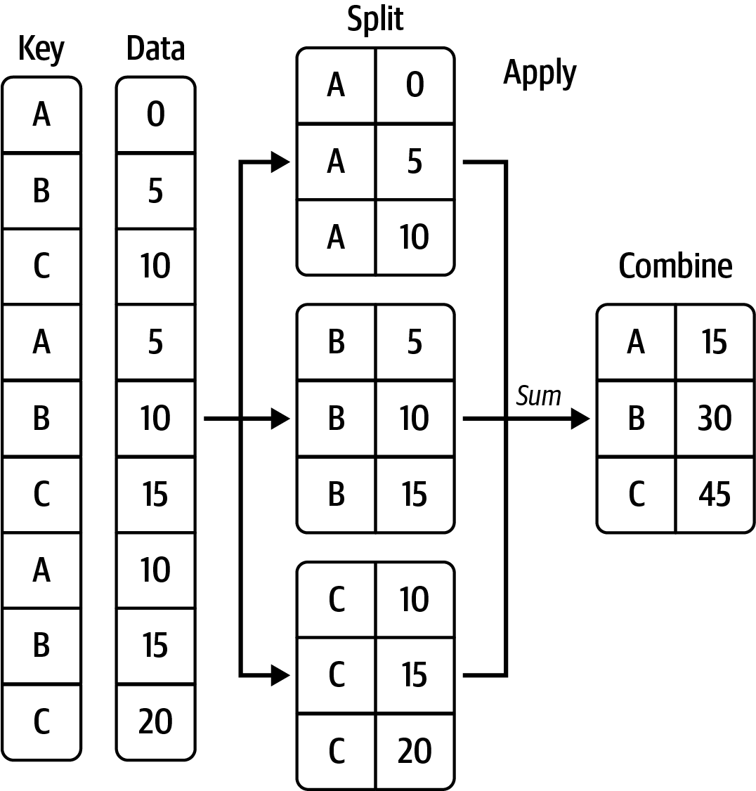
groupby(), agg(), apply()카테고리별로 나뉘어진 데이터에 대한 통계치를 생성
groupby()는 데이터를 의미있는 그룹으로 나누어 분석할 수 있도록 해줌.count(), .sum(), .mean(), .min(), .max()과 같은 통계치를 구하는 methods와 함께 효과적으로 자주 활용됨
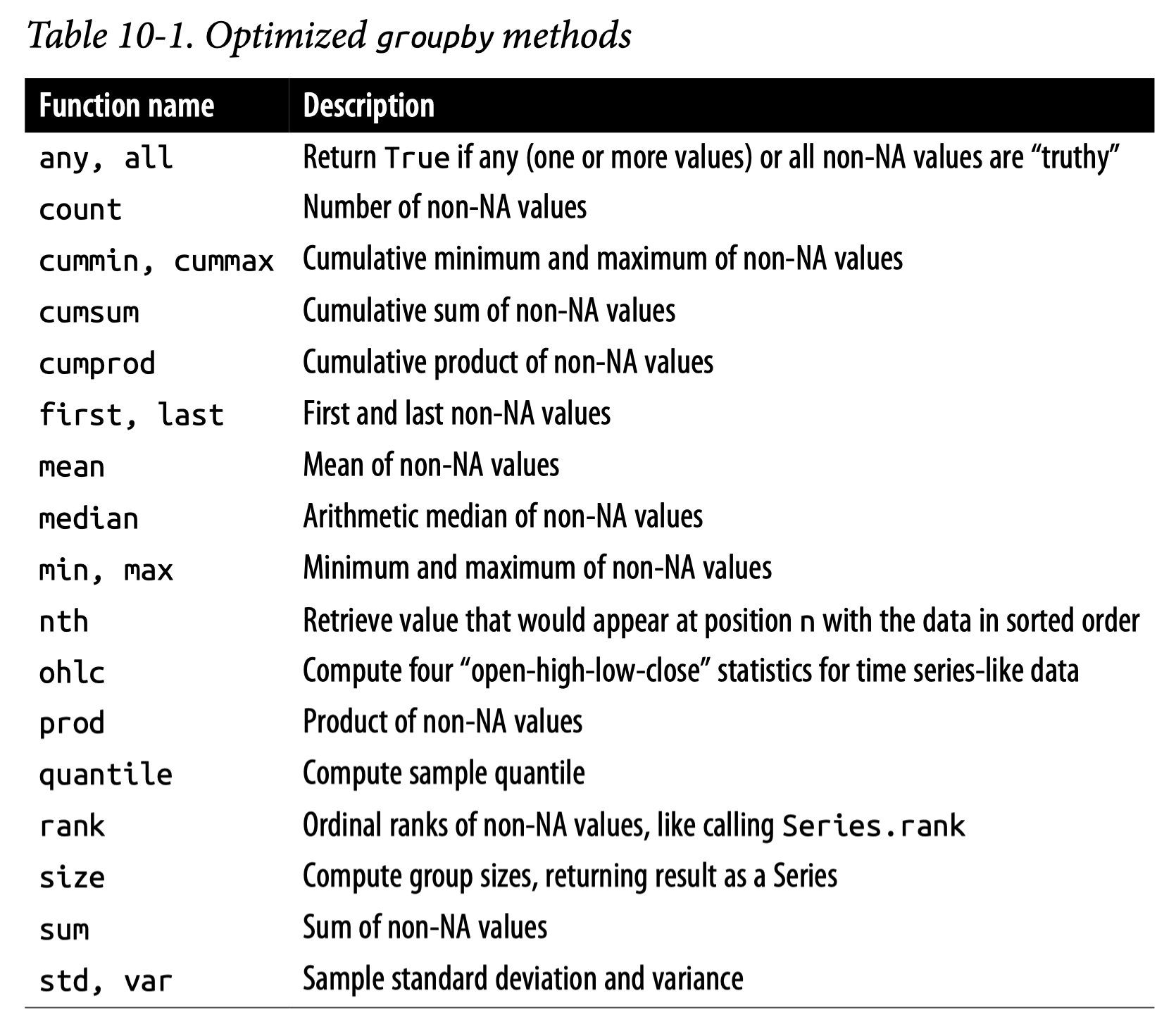
아래 표는 groupby()와 함께 자주 쓰이는 효율적인 methodsCh.10 in Python for Data Analysis (3e) by Wes McKinney
"movie_id" )["rating" ].mean()
movie_id
6      2.963
10     3.278
16     3.045
        ...
4483   3.192
4488   3.552
4492   2.657
Name: rating, Length: 844, dtype: Float64
"user_id" )["rating" ].agg(["mean" , "std" ])
user_id
6
3.200
0.414
7
4.067
1.033
10
3.500
1.732
...
...
...
2649401
4.200
1.095
2649426
3.667
0.577
2649429
4.000
0.894
336915 rows × 2 columns
def min_max(x):return pd.Series([x.min (), x.max ()], index= ["min" , "max" ]) # Series를 반환 "movie_id" )["rating" ].apply (min_max)
movie_id
6         min    1
          max    5
10        min    1
                ..
4488      max    5
4492      min    1
          max    5
Name: rating, Length: 1688, dtype: int8
def standardize_by_user(x):return (x - x.mean()) / x.std()"user_id" )["rating" ]apply (standardize_by_user)= 0 )
117541
6
-0.483
324856
6
1.932
412793
6
-0.483
...
...
...
1340788
2649429
1.118
1384493
2649429
-1.118
1683632
2649429
-1.118
1862726 rows × 2 columns
Exploratory Data Analysis (EDA)
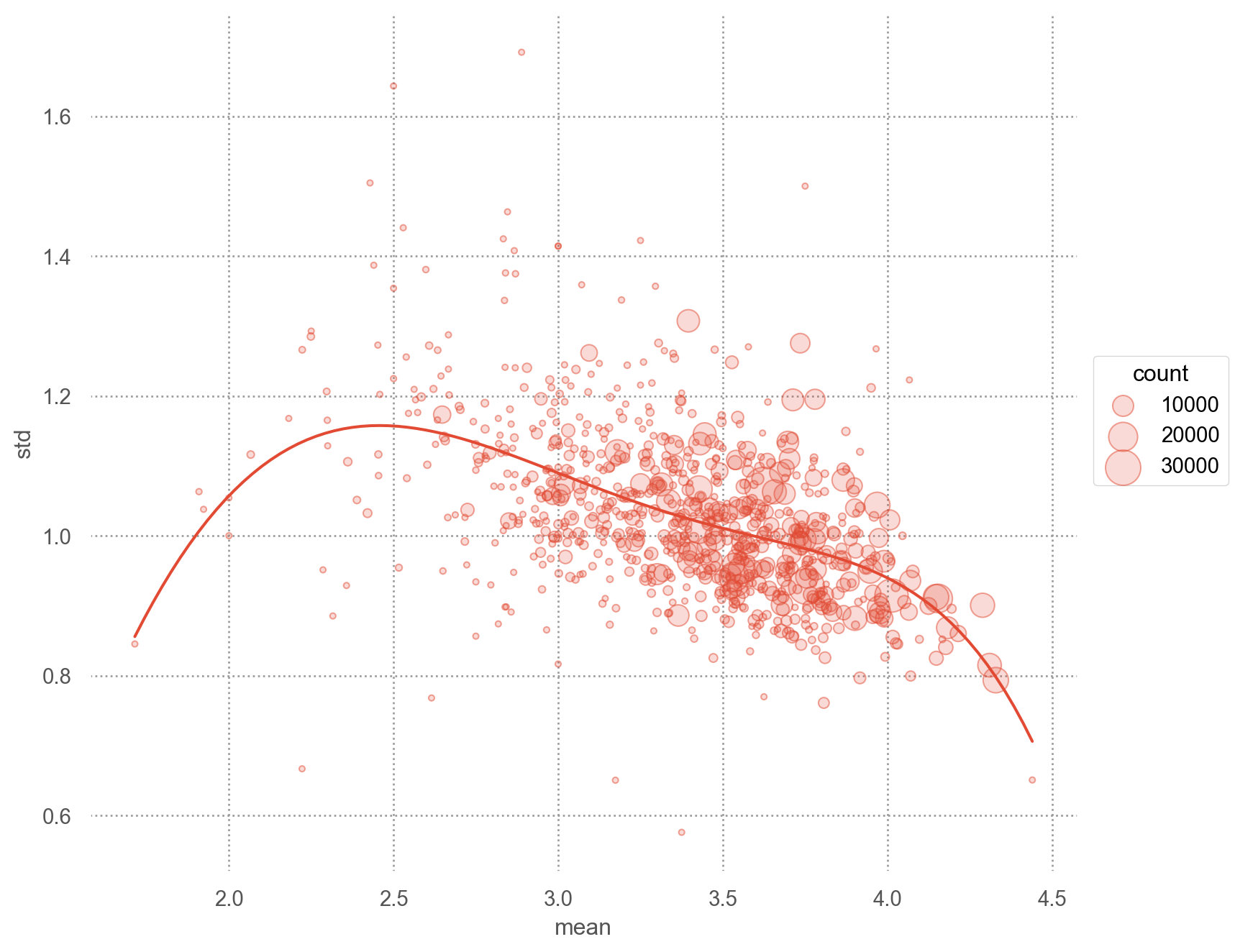
평점 분포
= ("title" )["rating" ] # title보다는 movie_id로 그룹화하는 것이 더 적절함 "mean" , "std" , "count" ])
0
10
3.104
0.956
498
1
10 Things I Hate About You
3.728
0.992
4705
2
11:14
3.203
1.030
266
...
...
...
...
...
822
Wrongfully Accused
3.290
1.143
252
823
Yellow Submarine
3.575
1.105
784
824
Youngblood
3.256
1.029
328
825 rows × 4 columns
"mean" , ascending= False )
430
Paradise Lost: The Child Murders at Robin Hood...
4.440
0.651
25
734
The Sixth Sense
4.329
0.793
15166
733
The Silence of the Lambs
4.310
0.815
12940
...
...
...
...
...
468
Red Riding Hood
1.923
1.038
13
476
Rhinestone
1.909
1.063
66
562
Stuck on You
1.714
0.845
21
825 rows × 4 columns
= "mean" , y= "std" )= .5 ), pointsize= "count" )5 ))= (3 , 20 ))= (8 , 7 ))
= (= lambda x: x["year" ] // 10 * 10 , # 10년 단위 = lambda x: x["date" ].dt.day_name().str [:3 ],= lambda x: x["weekday" ].isin(["Sat" , "Sun" ]),= lambda x: x["title" ].str .len ()"weekday" ] = netflix2["weekday" ].astype("category" ).cat.set_categories(["Mon" , "Tue" , "Wed" , "Thu" , "Fri" , "Sat" , "Sun" ])
0
3282
972104
4
2005-09-16
Sideways
[Comedy, Drama, Romance]
2004
2000
Fri
False
8
1
143
2297762
5
2004-08-07
The Game
[Drama, Mystery, Thriller]
1997
1990
Sat
True
8
2
1744
1489846
3
2003-05-22
Beverly Hills Cop
[Action, Comedy, Crime]
1984
1980
Thu
False
17
3
357
1169994
5
2004-04-22
House of Sand and Fog
[Crime, Drama]
2003
2000
Thu
False
21
4
3256
722964
3
2004-03-08
Swimming Pool
[Crime, Drama, Mystery]
2003
2000
Mon
False
13
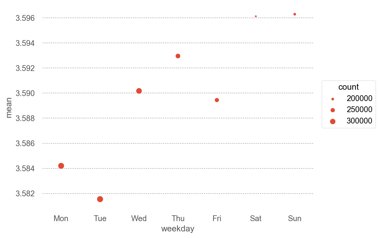
= ("weekday" ])["rating" ]"mean" , "std" , "count" ])
0
Mon
3.584
1.054
324006
1
Tue
3.582
1.054
331272
2
Wed
3.590
1.055
311012
3
Thu
3.593
1.057
267394
4
Fri
3.589
1.061
245186
5
Sat
3.596
1.065
184385
6
Sun
3.596
1.060
199471
요일별 평점
= "weekday" , y= "mean" )= "count" )
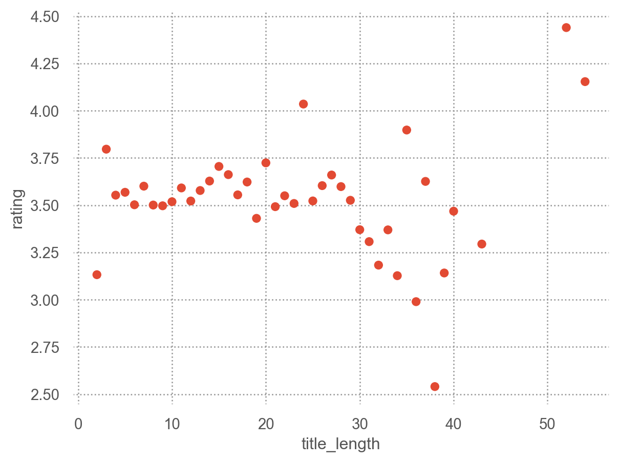
제목의 길이?
= "title_length" , y= "rating" )"mean" ))
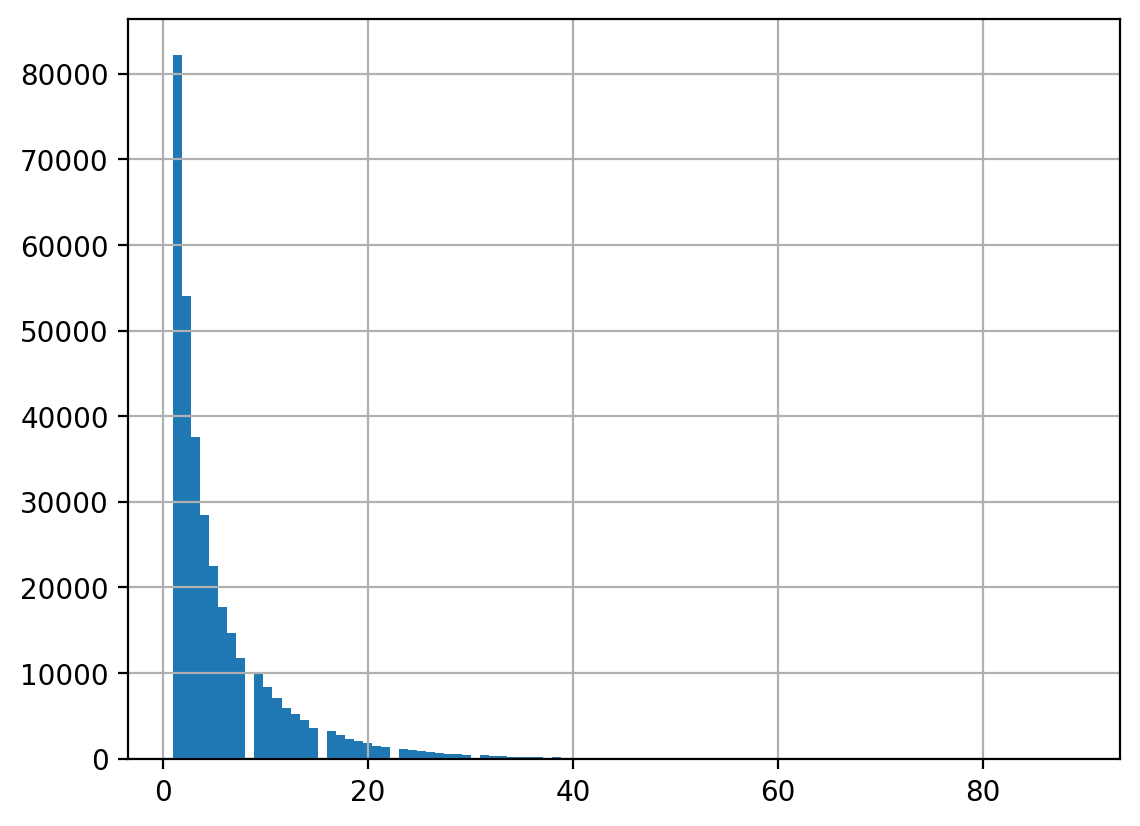
시청자별 분석
= netflix.groupby("user_id" )["rating" ].size()
user_id
6          15
7          15
10          4
           ..
2649401     5
2649426     3
2649429     6
Name: rating, Length: 336915, dtype: Int64
# pandas의 method를 사용한 시각화 = 100 );
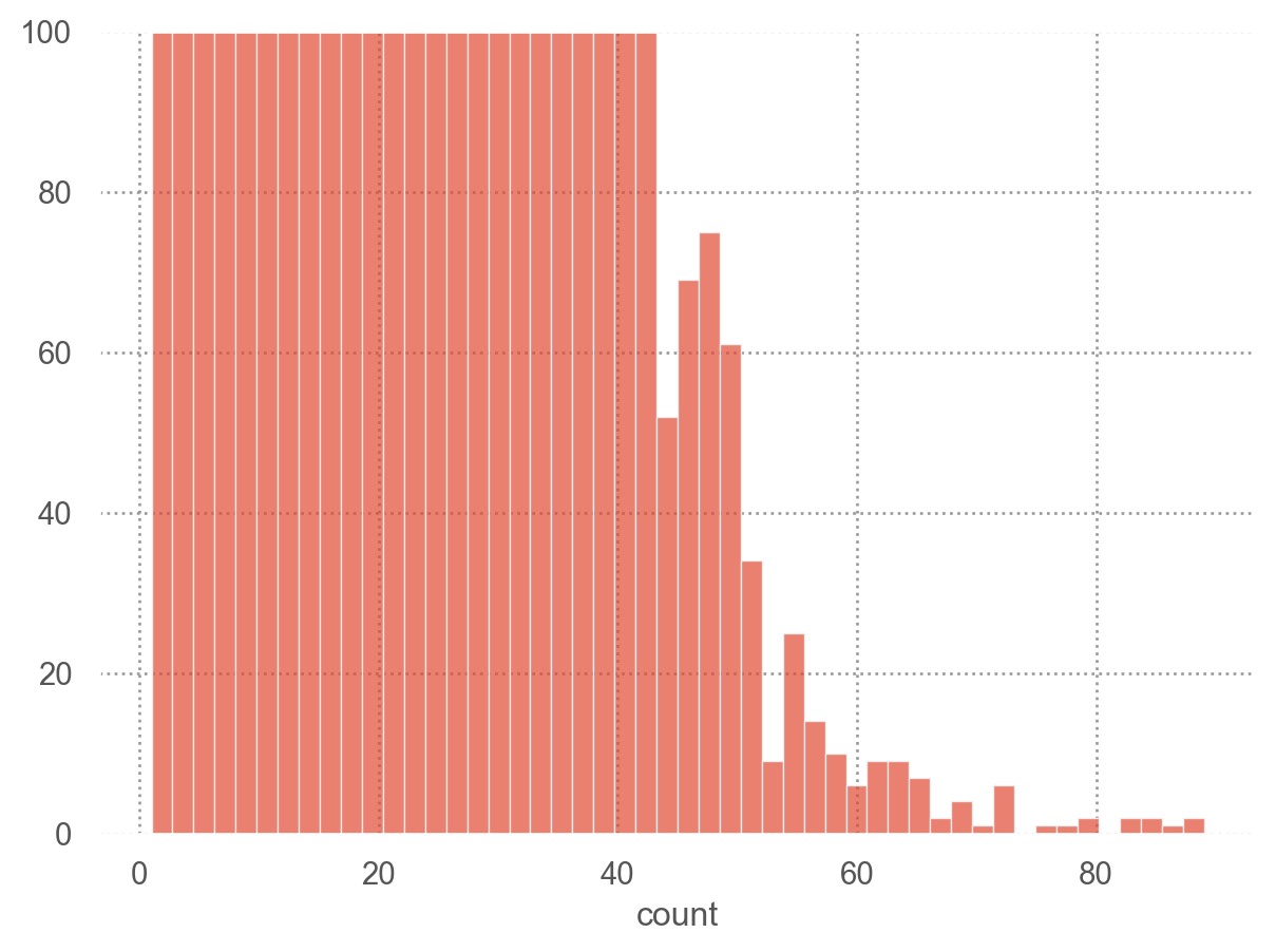
= viewing_count.reset_index(name= "count" )= "count" )= 50 ))= (0 , 100 ))
= ("user_id" )["rating" ]"mean" , "std" , "count" ])
user_id
6
3.200
0.414
15
7
4.067
1.033
15
10
3.500
1.732
4
...
...
...
...
2649401
4.200
1.095
5
2649426
3.667
0.577
3
2649429
4.000
0.894
6
336915 rows × 3 columns
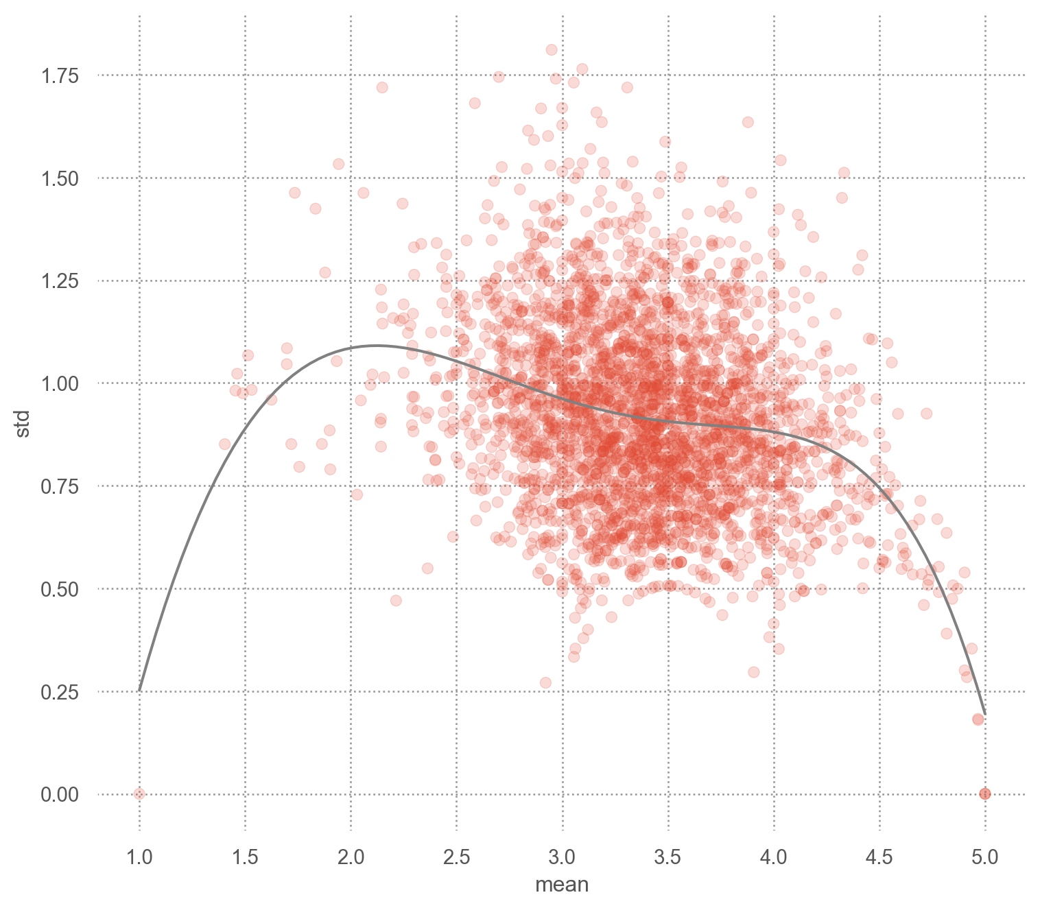
= user_stats.query("count >= 30" )
user_id
1333
2.674
0.778
43
2213
3.871
0.846
31
2455
3.433
0.817
30
...
...
...
...
2646574
3.119
0.803
42
2647197
3.389
1.153
36
2648287
3.600
0.847
35
3051 rows × 3 columns
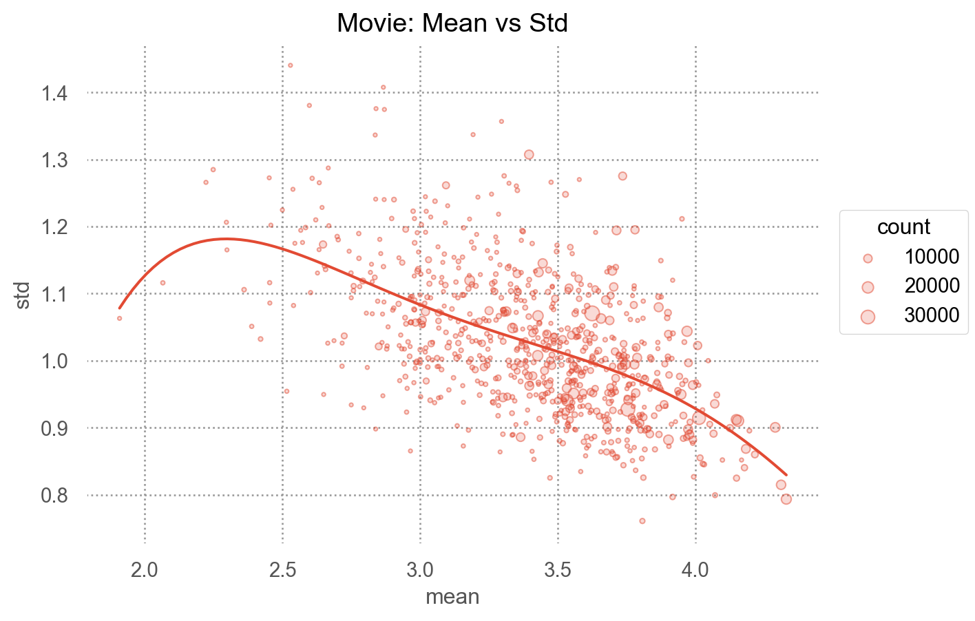
= "mean" , y= "std" )= .2 ))= ".5" ), so.PolyFit(5 ))= (8 , 7 ))
장르별 분석
0            [Comedy, Drama, Romance]
1          [Drama, Mystery, Thriller]
2             [Action, Comedy, Crime]
                      ...
1862723      [Drama, Horror, Mystery]
1862724       [Action, Comedy, Crime]
1862725       [Biography, Drama, War]
Name: genre, Length: 1862726, dtype: object
= netflix.explode('genre' )
0
3282
972104
4
2005-09-16
Sideways
Comedy
2004
0
3282
972104
4
2005-09-16
Sideways
Drama
2004
0
3282
972104
4
2005-09-16
Sideways
Romance
2004
...
...
...
...
...
...
...
...
1862725
2782
1465983
4
2005-06-22
Braveheart
Biography
1995
1862725
2782
1465983
4
2005-06-22
Braveheart
Drama
1995
1862725
2782
1465983
4
2005-06-22
Braveheart
War
1995
4806517 rows × 7 columns
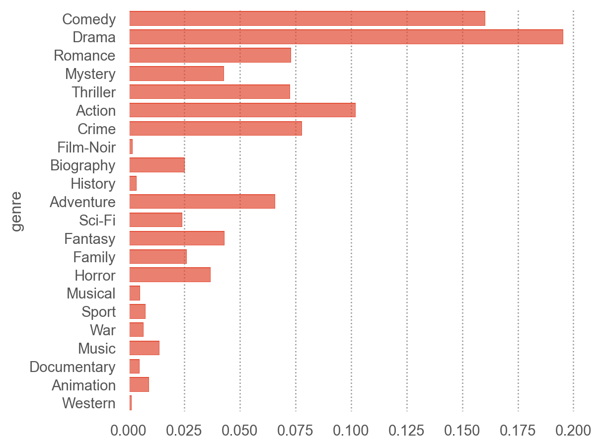
= "genre" ) # y에 genre가 나오도록! "proportion" ))
= ('genre' )['rating' ]'mean' , 'std' , 'count' ])
0
Action
3.557
1.050
490601
1
Adventure
3.576
1.064
316881
2
Animation
3.811
1.018
44297
...
...
...
...
...
19
Thriller
3.620
1.030
348897
20
War
3.908
1.037
32304
21
Western
3.577
1.045
6361
22 rows × 4 columns
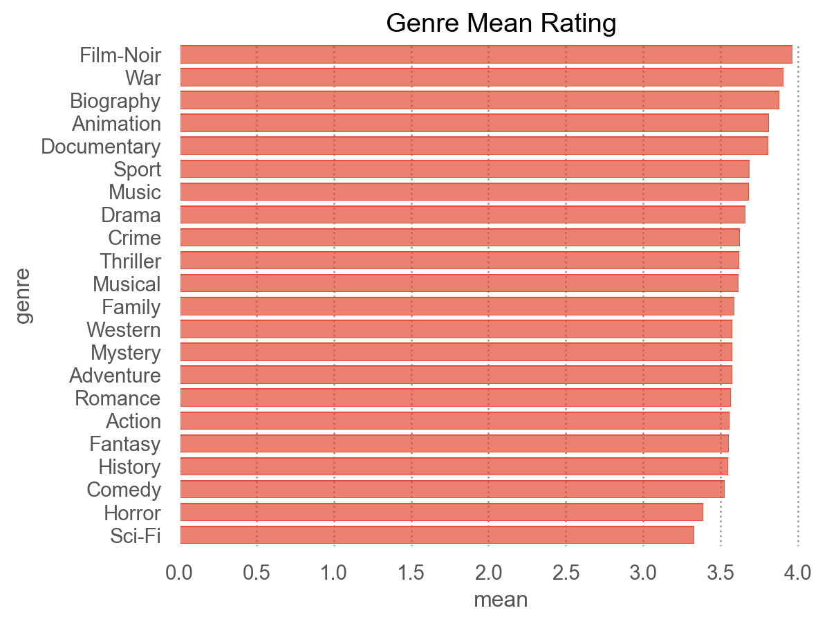
3 , "mean" )
10
Film-Noir
3.965
0.935
9020
20
War
3.908
1.037
32304
3
Biography
3.878
0.995
121688
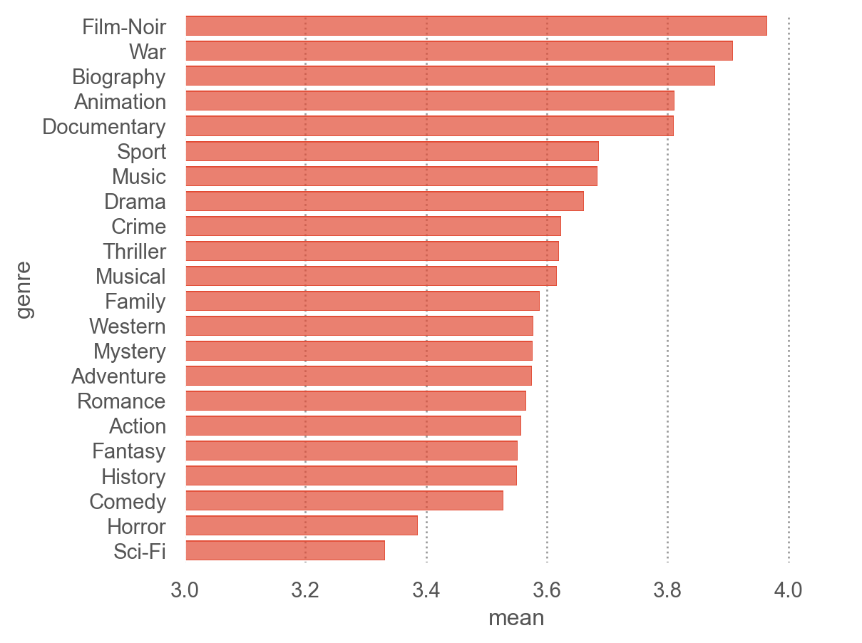
= genre_mean.sort_values("mean" , ascending= False )["genre" ].values= "genre" , x= "mean" )= so.Nominal(order= order_by_mean)) # 그래프에 순서 부여 = (3 , 4.1 ))
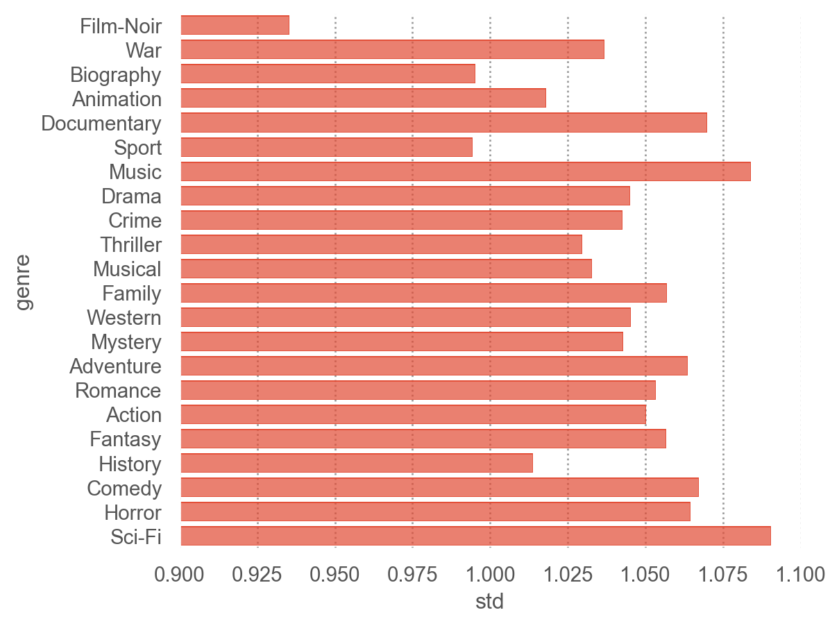
= "genre" , x= "std" )= so.Nominal(order= order_by_mean)) # 그래프에 순서 부여 = (.9 , 1.1 ))
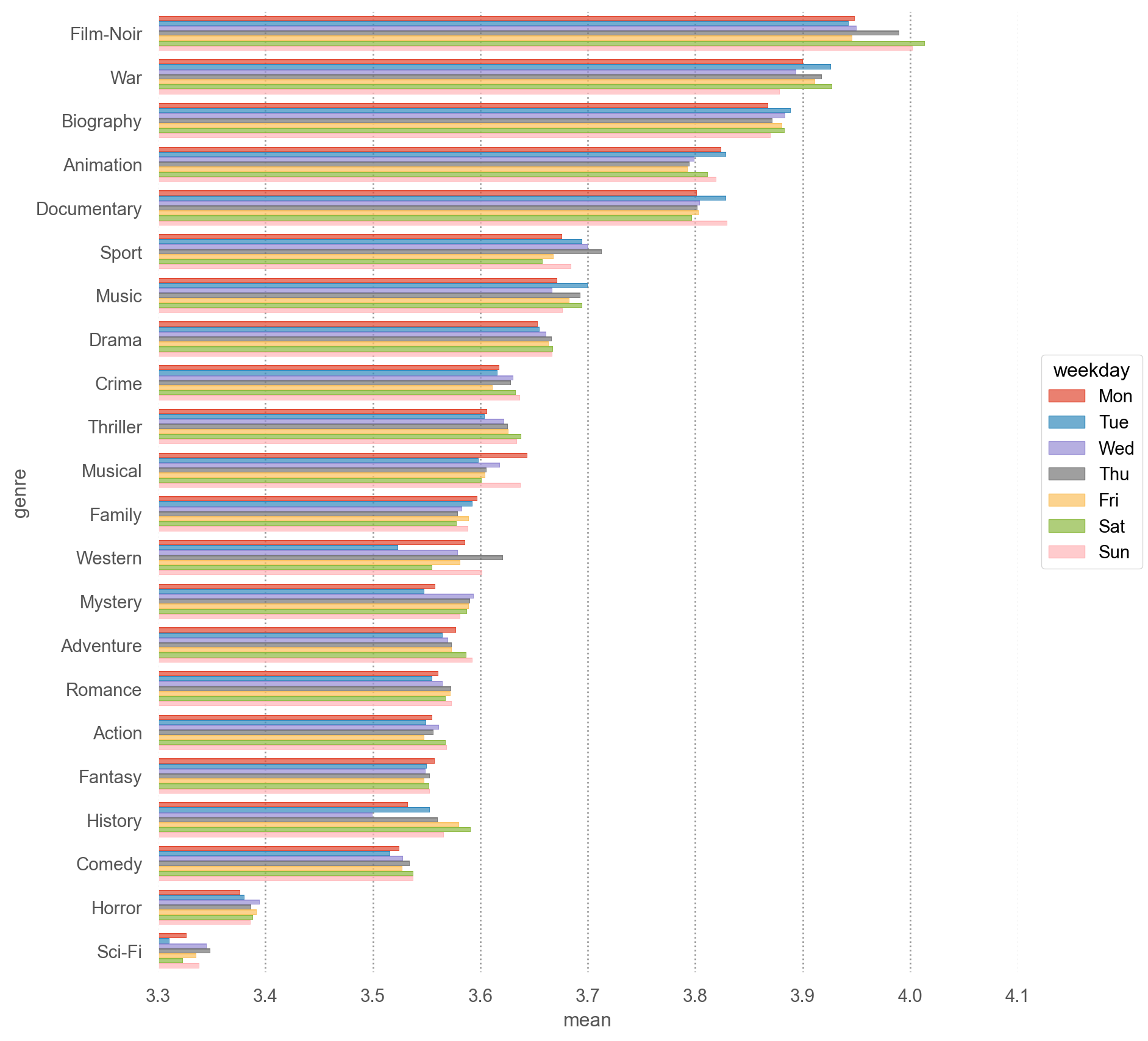
"weekday" ] = netflix_long["date" ].dt.day_name().str [:3 ]"weekday" ] = netflix_long["weekday" ].astype("category" ).cat.set_categories(["Mon" , "Tue" , "Wed" , "Thu" , "Fri" , "Sat" , "Sun" ])= ('genre' , 'weekday' ], observed= True )['rating' ]'mean' , 'std' , 'count' ])
0
Action
Mon
3.555
1.045
85715
1
Action
Tue
3.549
1.043
86670
2
Action
Wed
3.561
1.047
82093
...
...
...
...
...
...
151
Western
Fri
3.581
1.034
836
152
Western
Sat
3.555
1.015
632
153
Western
Sun
3.602
0.997
738
154 rows × 5 columns
= genre_mean.sort_values("mean" , ascending= False )["genre" ].values= "genre" , x= "mean" , color= "weekday" )= so.Nominal(order= order_by_mean)) # 그래프에 순서 부여 # .facet("weekday") = (3.3 , 4.1 ))= (9 , 9 ))
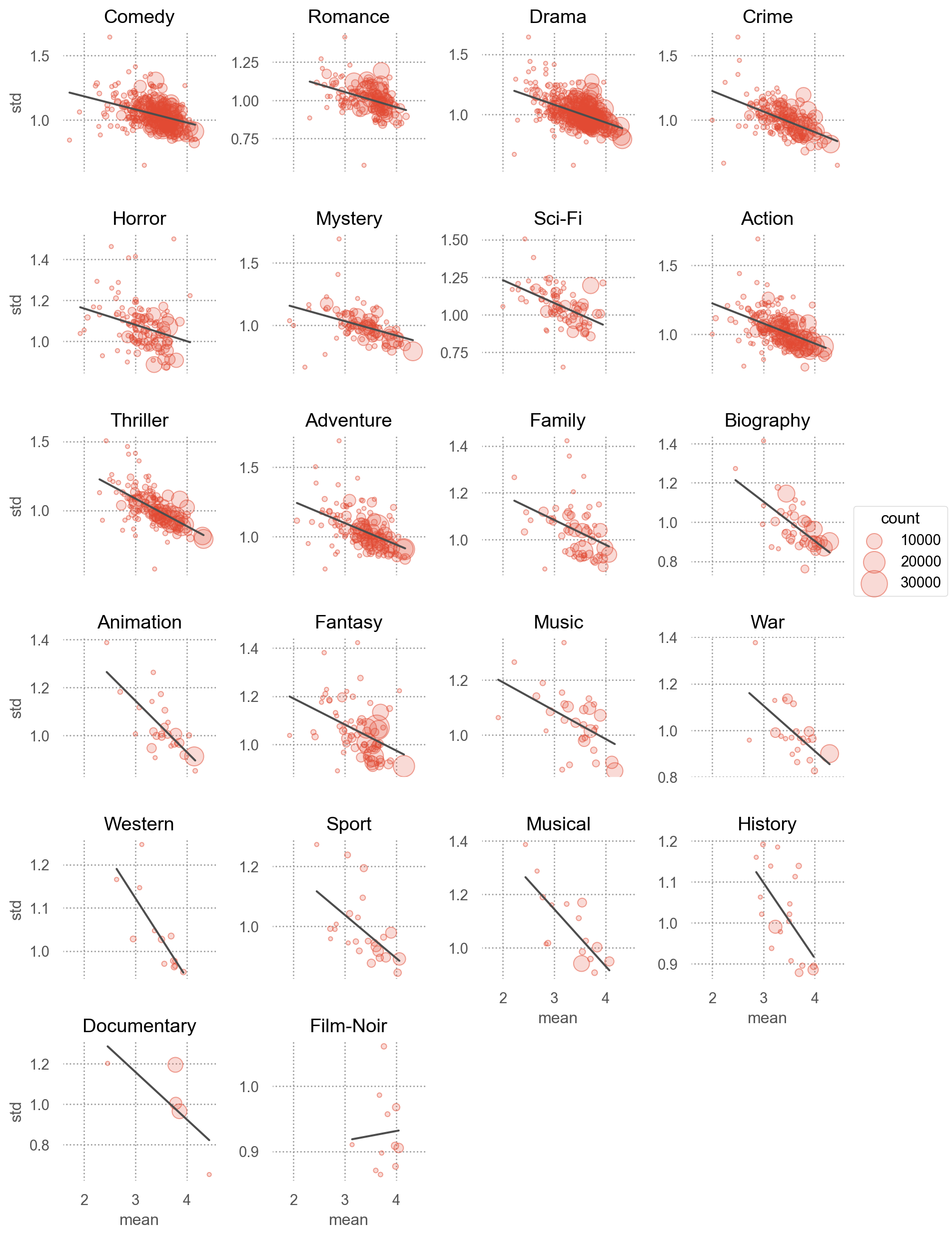
= ("title" , "genre" ])["rating" ]"mean" , "std" , "count" ])
0
10
Comedy
3.104
0.956
498
1
10
Romance
3.104
0.956
498
2
10 Things I Hate About You
Comedy
3.728
0.992
4705
...
...
...
...
...
...
2201
Youngblood
Drama
3.256
1.029
328
2202
Youngblood
Romance
3.256
1.029
328
2203
Youngblood
Sport
3.256
1.029
328
2204 rows × 5 columns
= "mean" , y= "std" )= .5 ), pointsize= "count" )= ".3" ), so.PolyFit(1 ))"genre" , wrap= 4 )= False )= (3 , 20 ))= (9 , 13 ))
출시년도
0
3282
972104
4
2005-09-16
Sideways
[Comedy, Drama, Romance]
2004
1
143
2297762
5
2004-08-07
The Game
[Drama, Mystery, Thriller]
1997
2
1744
1489846
3
2003-05-22
Beverly Hills Cop
[Action, Comedy, Crime]
1984
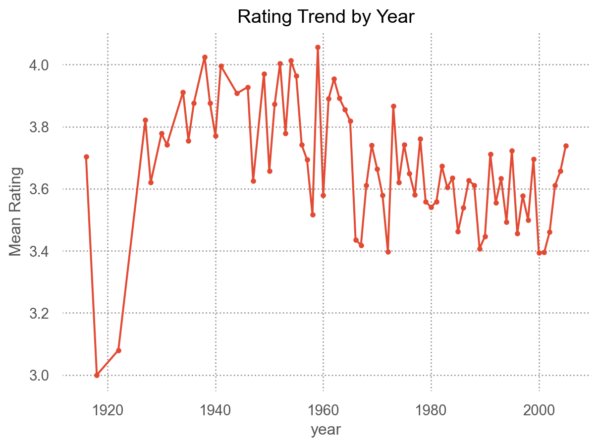
"year" , "title" ])["rating" ].agg(["mean" , "count" ])
year
title
1916
20,000 Leagues Under the Sea
3.704
162
1918
Chaplin
3.000
47
1922
Robin Hood
3.080
75
...
...
...
...
2005
The Hitchhiker's Guide to the Galaxy
2.997
2949
The Pacifier
3.580
3966
Unleashed
3.733
845
844 rows × 2 columns
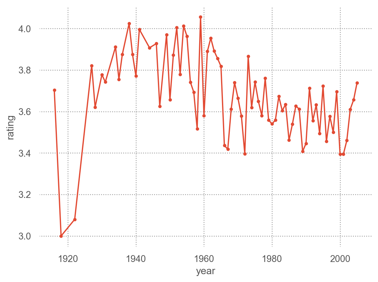
= "year" , y= "rating" )= "." ), so.Agg("mean" ))
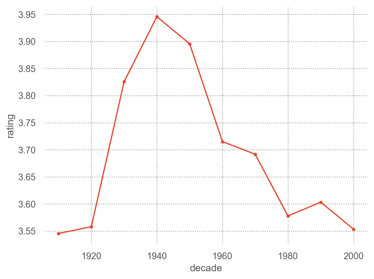
# 10년 단위로 "decade" ] = netflix["year" ] // 10 * 10 = "decade" , y= "rating" )= "." ), so.Agg("mean" ))
Module로 변환/활용
반복되는 분석 패턴을 netflix_utils.py 모듈로 분리하고 함수들을 정의
import netflix_utils as nu
import netflix_utils as nu# 데이터 로딩 및 환경 설정 = 6 )= nu.load_netflix_data("data/netflix_ratings.parquet" )3 )
0
3282
972104
4
2005-09-16
Sideways
[Comedy, Drama, Romance]
2004
1
143
2297762
5
2004-08-07
The Game
[Drama, Mystery, Thriller]
1997
2
1744
1489846
3
2003-05-22
Beverly Hills Cop
[Action, Comedy, Crime]
1984
# 파생 변수 한 번에 추가 (decade, weekday, title_length) = nu.enrich_netflix(netflix)3 )
0
3282
972104
4
2005-09-16
Sideways
[Comedy, Drama, Romance]
2004
2000
Fri
8
1
143
2297762
5
2004-08-07
The Game
[Drama, Mystery, Thriller]
1997
1990
Sat
8
2
1744
1489846
3
2003-05-22
Beverly Hills Cop
[Action, Comedy, Crime]
1984
1980
Thu
17
# 영화별 통계 (최소 30명 이상 평가한 영화만) = nu.movie_stats(netflix, min_count= 30 )"mean" , ascending= False ).head()
734
The Sixth Sense
4.329
0.793
15166
733
The Silence of the Lambs
4.310
0.815
12940
101
Braveheart
4.289
0.901
13590
72
Batman Begins
4.215
0.860
5529
510
Sense and Sensibility
4.195
0.896
1133
# 사용자별 통계 (최소 30개 이상 평가한 사용자만) = nu.user_stats(netflix, min_count= 30 )
user_id
1333
2.674
0.778
43
2213
3.871
0.846
31
2455
3.433
0.817
30
2905
3.700
1.418
30
3321
2.977
1.012
43
# 장르별 통계 = nu.genre_stats(netflix)"mean" , ascending= False )
10
Film-Noir
3.965
0.935
9020
20
War
3.908
1.037
32304
3
Biography
3.878
0.995
121688
...
...
...
...
...
4
Comedy
3.528
1.067
770697
12
Horror
3.386
1.065
177556
17
Sci-Fi
3.332
1.090
115480
22 rows × 4 columns
# 범용 집계: 요일별 평점 = nu.add_ordered_weekday(netflix)"weekday" )
0
Mon
3.584
1.054
324006
1
Tue
3.582
1.054
331272
2
Wed
3.590
1.055
311012
...
...
...
...
...
4
Fri
3.589
1.061
245186
5
Sat
3.596
1.065
184385
6
Sun
3.596
1.060
199471
7 rows × 4 columns
# 시각화: 평균 vs 표준편차 산점도 = "Movie: Mean vs Std" )
# 시각화: 장르 순위 = "mean" , title= "Genre Mean Rating" )
# 시각화: 연도별 평점 추세 = "year" , title= "Rating Trend by Year" )
# 사용자별 평점 표준화 (z-score) = nu.standardize_rating_by(netflix, group_col= "user_id" )
117541
6
-0.483
324856
6
1.932
412793
6
-0.483
448624
6
1.932
604841
6
-0.483