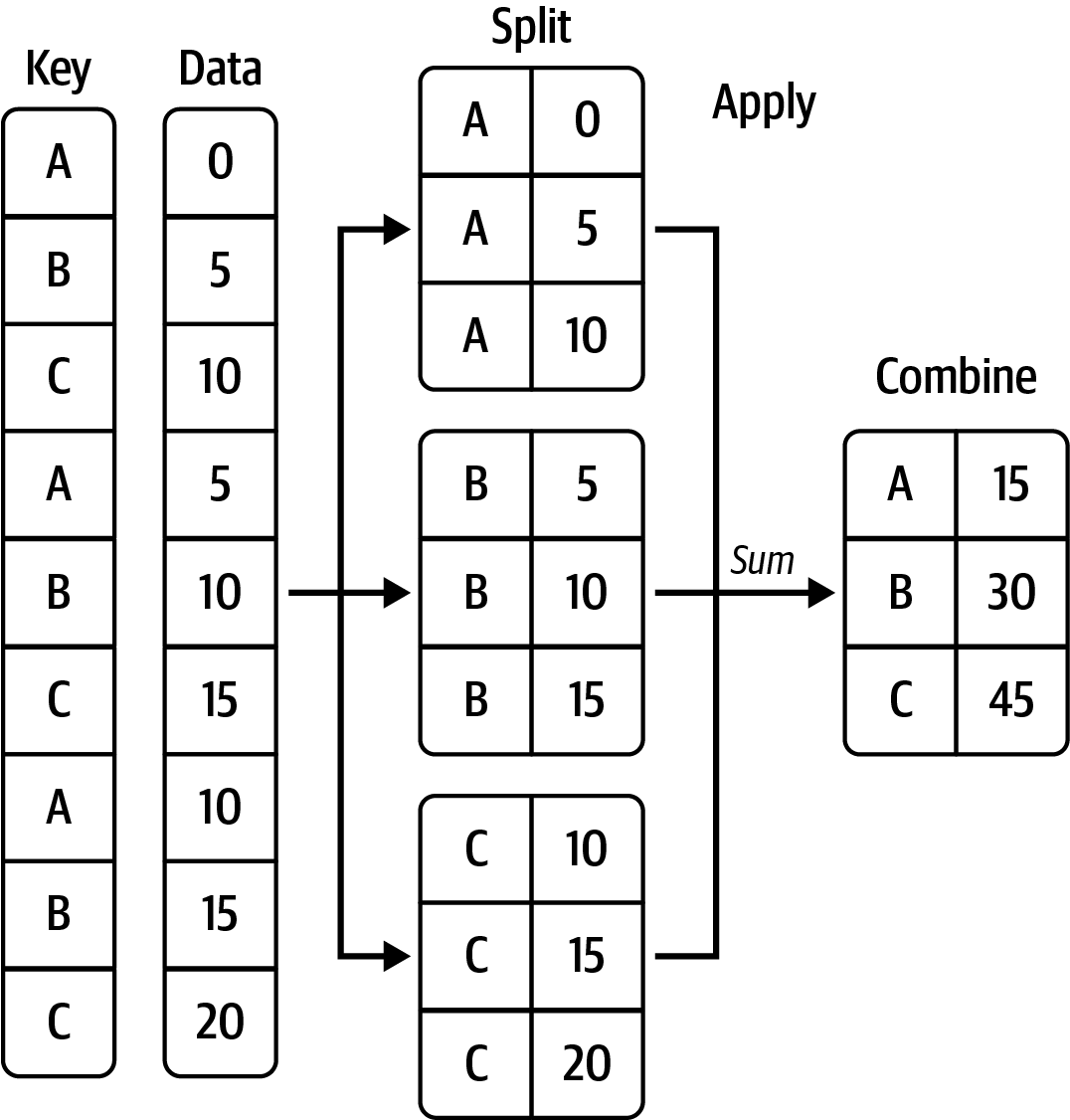
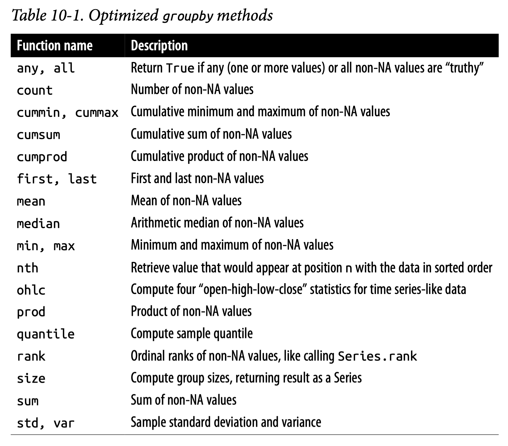
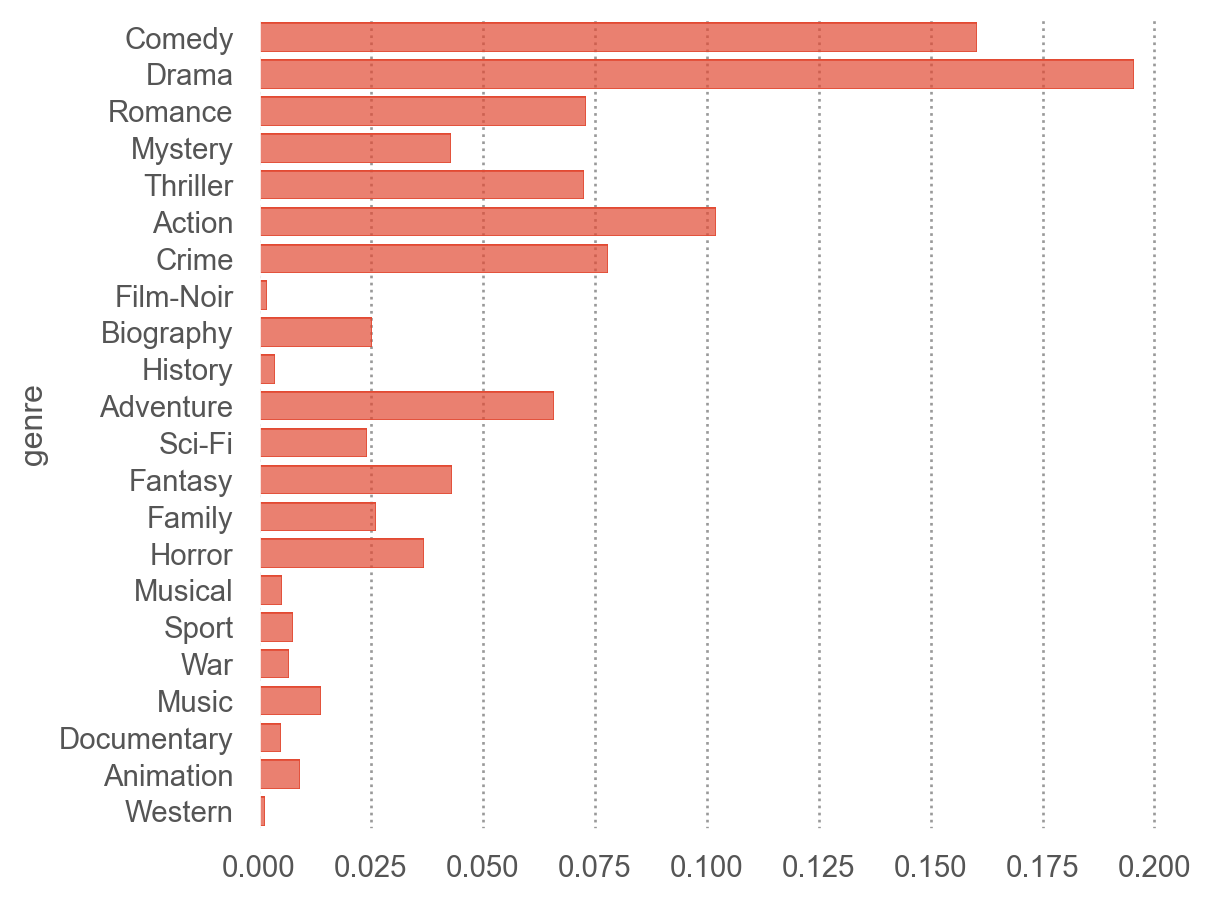
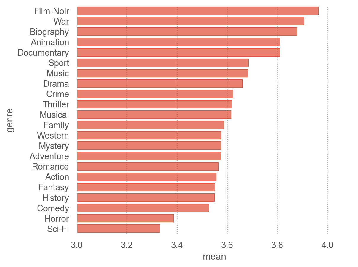
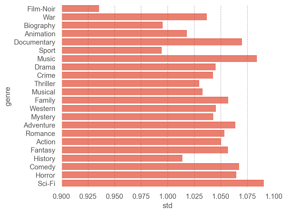
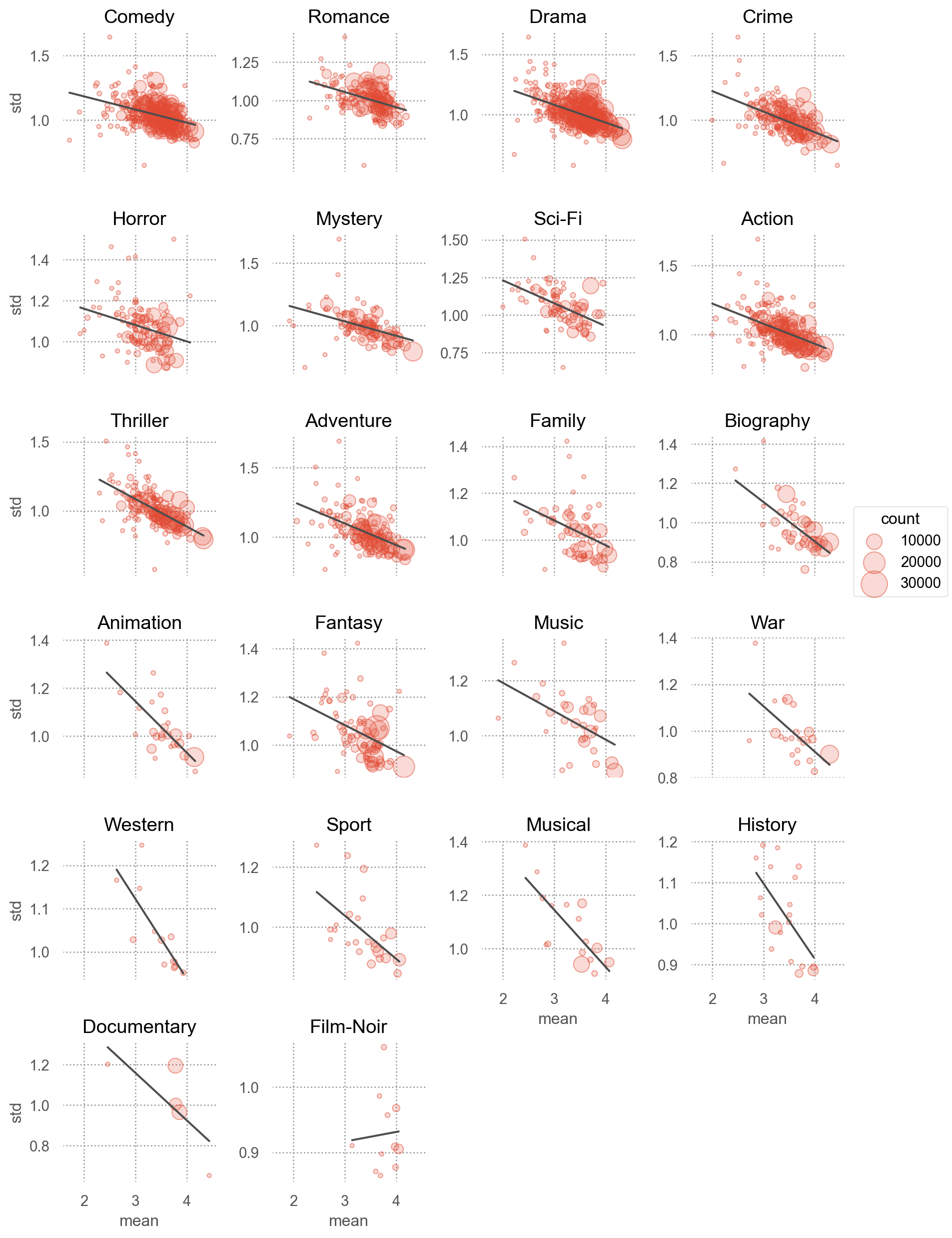
카테고리별로 나뉘어진 데이터에 대한 통계치를 생성: groupby(), agg(), apply()
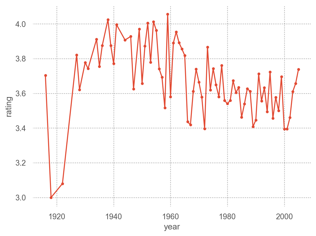
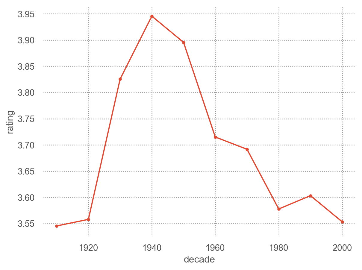
netflix_1990 = ( netflix .loc[:, ["title", "rating", "date", "year"]] # 특정 열을 선택 .query("year >= 1990") # 조건에 맞는 행만 필터링 .assign( # 새로운 열/변수를 생성 decade=lambda x: x["year"] //10*10, # 10년 단위 weekday=lambda x: x["date"].dt.day_name().str[:3] # 요일 ) .sort_values("year") # 조건에 따라 행을 정렬)netflix_1990
title
rating
date
year
decade
weekday
150148
Flatliners
3
2004-08-14
1990
1990
Sat
1269856
Look Who's Talking Too
3
2004-09-24
1990
1990
Fri
562709
Ghost
2
2004-12-28
1990
1990
Tue
1667117
The Grifters
3
2005-05-15
1990
1990
Sun
1269834
Ghost
4
2002-03-01
1990
1990
Fri
...
...
...
...
...
...
...
456802
Beauty Shop
5
2005-10-22
2005
2000
Sat
608408
Hostage
4
2005-10-10
2005
2000
Mon
456776
Hostage
5
2005-07-18
2005
2000
Mon
1818277
Coach Carter
4
2005-08-03
2005
2000
Wed
519199
The Hitchhiker's Guide to the Galaxy
3
2005-11-22
2005
2000
Tue
1496107 rows × 6 columns
subsetting
변수들(열)과 관측치(행)를 선택
Bracket []
Dot-notation .
iloc, loc
표시줄 수 지정
# max number of rows to displaypd.options.display.max_rows =7# resetpd.options.display.max_rows =0
Conditional operators
>, >=, <, <=,
== (equal to), != (not equal to) and, & (and) or, | (or) not, ~ (not) in (includes), not in (not included)
netflix.query("year >= 1990 & year < 2000")
movie_id
user_id
rating
date
title
genre
year
1
143
2297762
5
2004-08-07
The Game
[Drama, Mystery, Thriller]
1997
8
3730
619966
4
2005-06-01
Elizabeth
[Biography, Drama, History]
1998
12
571
637726
4
2005-02-15
American Beauty
[Drama]
1999
...
...
...
...
...
...
...
...
1862722
3782
1550938
3
2005-02-07
Flatliners
[Drama, Horror, Sci-Fi]
1990
1862723
3782
1550938
3
2005-02-07
Flatliners
[Drama, Horror, Mystery]
1990
1862725
2782
1465983
4
2005-06-22
Braveheart
[Biography, Drama, War]
1995
578142 rows × 7 columns
netflix.query("rating in [1, 5]")
movie_id
user_id
rating
date
title
genre
year
1
143
2297762
5
2004-08-07
The Game
[Drama, Mystery, Thriller]
1997
3
357
1169994
5
2004-04-22
House of Sand and Fog
[Crime, Drama]
2003
11
3798
2186643
5
2004-10-01
The Sting
[Comedy, Crime, Drama]
1973
...
...
...
...
...
...
...
...
1862715
3890
1690697
1
2005-07-12
Confessions of a Teenage Drama Queen
[Comedy, Family, Music]
2004
1862716
1905
528664
5
2005-10-06
Pirates of the Caribbean: The Curse of the Bla...
[Action, Adventure, Fantasy]
2003
1862718
1144
434884
5
2005-07-28
Fried Green Tomatoes
[Drama]
1991
473038 rows × 7 columns
# title에 game이 포함되어 있는 행만 필터링netflix.loc[netflix.title.str.contains("Game"), :] # .str: 문자열 처리# 동일한 작업을 query()를 이용해 필터링netflix.query("title.str.contains('Game')")
movie_id
user_id
rating
date
title
genre
year
1
143
2297762
5
2004-08-07
The Game
[Drama, Mystery, Thriller]
1997
81
143
147712
4
2005-03-11
The Game
[Drama, Mystery, Thriller]
1997
428
3703
2147997
4
2004-08-24
Ripley's Game
[Crime, Drama, Mystery]
2003
...
...
...
...
...
...
...
...
1862313
143
702062
5
2004-09-26
The Game
[Drama, Mystery, Thriller]
1997
1862403
1329
2581467
3
2005-06-13
He Got Game
[Drama, Sport]
1998
1862604
1329
1684165
3
2004-11-03
He Got Game
[Drama, Sport]
1998
7318 rows × 7 columns
sort_values()
조건에 맞도록 행을 재정렬
netflix.sort_values("year") # year에 대해 오름차순 정렬netflix.sort_values("year", ascending=False) # year에 대해 내림차순 정렬netflix.sort_values(["year", "rating"], ascending=False) # year 다음 rating에 대해 내림차순 정렬
movie_id
user_id
rating
date
title
genre
year
26
1073
1628274
5
2005-09-14
Coach Carter
[Biography, Drama, Sport]
2005
747
3689
818707
5
2005-05-07
The Amityville Horror
[Horror]
2005
766
3864
492243
5
2005-11-25
Batman Begins
[Action, Crime, Drama]
2005
...
...
...
...
...
...
...
...
1194696
394
1297880
1
2003-10-26
20,000 Leagues Under the Sea
[Adventure, Drama, Family]
1916
1290064
394
909041
1
2002-08-18
20,000 Leagues Under the Sea
[Adventure, Drama, Family]
1916
1387785
394
344274
1
2005-07-22
20,000 Leagues Under the Sea
[Adventure, Drama, Family]
1916
1862726 rows × 7 columns
assign()
변수들과 함수들을 이용하여 새로운 변수를 생성
가령, 1990년대, 2000년대 등등과 같이 10년 단위로 새로운 값을 생성하려면,
netflix["year"] # pandas Series 객체, 그 값들은 NumPy array
패키지에서는 데이터를 한 번 담은 객체를 만들고, 그 객체에 .top_movies(), .genre_summary() 같은 메시지를 보냄
from_path()는 경로에서 바로 분석기를 만들어 주는 대체 생성자임.
# 경로에서 바로 분석기 생성 (load + 검증 + 파생변수 준비)analyzer = na.NetflixAnalyzer.from_path("data/netflix_ratings.parquet")print(analyzer) # __repr__ 가 보여 주는 요약analyzer.summary() # 데이터 규모 요약 딕셔너리
def analyze(data, cfg: AnalysisConfig):
    ...  # cfg.top_n, cfg.min_movie_ratings 등으로 깔끔하게 접근
설정값이 6개든 10개든, 함수에는 cfg 하나만 넘기면 됨
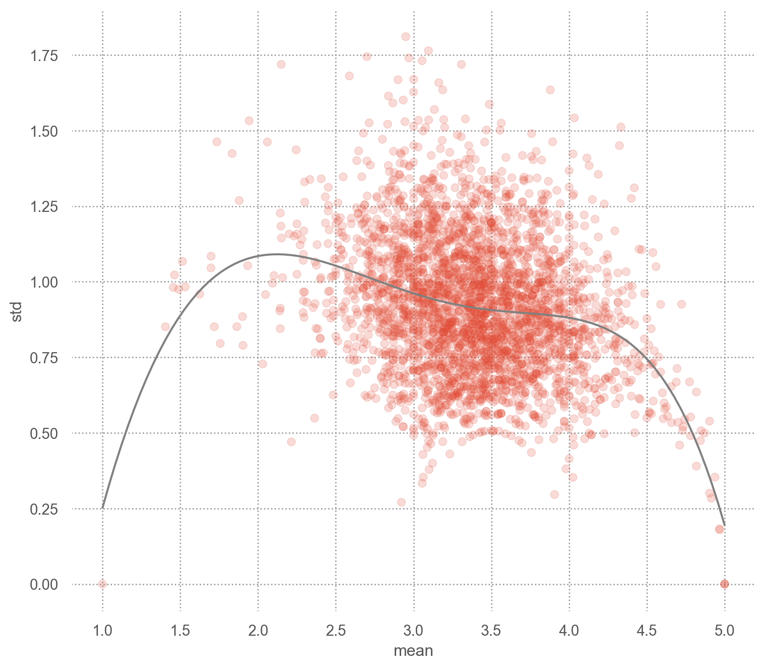
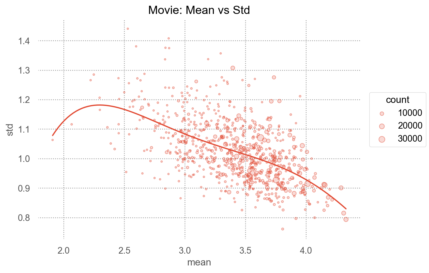
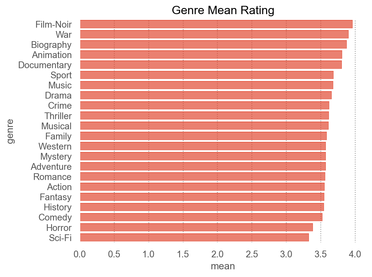
# 더 엄격한 기준: 1000명 이상이 평가한 영화만, Top 7strict = na.AnalysisConfig(min_movie_ratings=1000, top_n=7)analyzer_strict = na.NetflixAnalyzer(analyzer.data, config=strict)analyzer_strict.top_movies()
mean
std
count
title
The Sixth Sense
4.329
0.793
15166
The Silence of the Lambs
4.310
0.815
12940
Braveheart
4.289
0.901
13590
...
...
...
...
Sense and Sensibility
4.195
0.896
1133
Ray
4.182
0.868
11029
North by Northwest
4.177
0.840
4231
7 rows × 3 columns
# 잘못된 설정은 객체 생성 시점에 바로 걸러진다try: na.AnalysisConfig(top_n=-1)exceptValueErroras e:print("설정 오류:", e)
설정 오류: top_n은 양수여야 합니다: -1
.pipe(): 변환 함수를 체이닝하기
파생 변수 생성 단계를 작은 함수로 나누고, pandas의 .pipe() 메서드로 순서대로 연결.
각 함수는 df를 받아 df를 돌려주므로 체이닝이 가능하고, 필요한 변환만 골라 조합할 수도 있음.
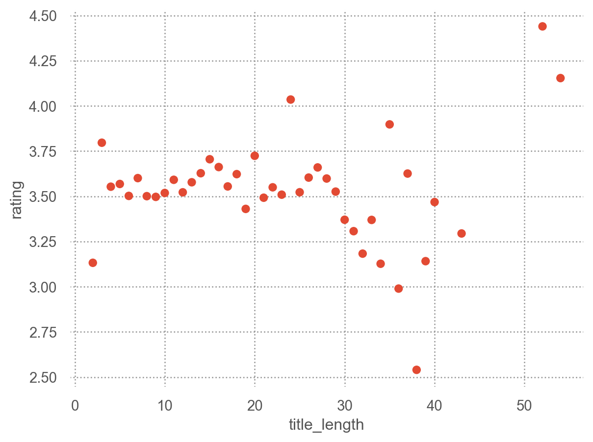
raw = analyzer._raw# 1) 개별 .pipe() 체이닝: 필요한 변환만 골라서 조합( raw .pipe(na.add_decade) # 연도 → 10년 단위 .pipe(na.add_title_length) # 제목 글자 수 .loc[:, ["title", "year", "decade", "title_length"]])
title
year
decade
title_length
0
Sideways
2004
2000
8
1
The Game
1997
1990
8
2
Beverly Hills Cop
1984
1980
17
...
...
...
...
...
1862723
Flatliners
1990
1990
10
1862724
Rush Hour 2
2001
2000
11
1862725
Braveheart
1995
1990
10
1862726 rows × 4 columns
# 2) 4개 변환 모두 조합( raw .pipe(na.add_decade) .pipe(na.add_ordered_weekday) .pipe(na.add_title_length) .pipe(na.normalize_genre) .loc[:, ["title", "year", "decade", "weekday", "title_length", "genre"]])
title
year
decade
weekday
title_length
genre
0
Sideways
2004
2000
Fri
8
[Comedy, Drama, Romance]
1
The Game
1997
1990
Sat
8
[Drama, Mystery, Thriller]
2
Beverly Hills Cop
1984
1980
Thu
17
[Action, Comedy, Crime]
...
...
...
...
...
...
...
1862723
Flatliners
1990
1990
Mon
10
[Drama, Horror, Mystery]
1862724
Rush Hour 2
2001
2000
Mon
11
[Action, Comedy, Crime]
1862725
Braveheart
1995
1990
Wed
10
[Biography, Drama, War]
1862726 rows × 6 columns
# 3) 위와 동일 — enrich()는 위 .pipe() 체이닝을 함수 하나로 묶은 것na.enrich(raw).loc[:, ["title", "year", "decade", "weekday", "title_length", "genre"]]
title
year
decade
weekday
title_length
genre
0
Sideways
2004
2000
Fri
8
[Comedy, Drama, Romance]
1
The Game
1997
1990
Sat
8
[Drama, Mystery, Thriller]
2
Beverly Hills Cop
1984
1980
Thu
17
[Action, Comedy, Crime]
...
...
...
...
...
...
...
1862723
Flatliners
1990
1990
Mon
10
[Drama, Horror, Mystery]
1862724
Rush Hour 2
2001
2000
Mon
11
[Action, Comedy, Crime]
1862725
Braveheart
1995
1990
Wed
10
[Biography, Drama, War]
1862726 rows × 6 columns
reporting: 분석과 표현의 분리
분석(NetflixAnalyzer)과 결과 표현(reporting)의 기능을 나눠 두면, 같은 분석 결과를 마크다운, HTML, PDF 등 다양한 형태로 재활용할 수 있음.
from IPython.display import Markdownreport = na.build_markdown_report(analyzer, top_n=5)Markdown(report) # markdown 형식으로 출력